
NUMERICAL METHODS
NUMERICAL METHODS
AND PROGRAMMING
AND PROGRAMMING
METHODS OF SOLVING
METHODS OF SOLVING
NONLINEAR EQUATIONS
Joanna Iwaniec
Root finding problem
Many problems in science and engineering are expressed as:
0
such that
value
the
find
,
function
continuous
a
Given
=
f(r)
r
f(x)
These problems are called root finding problems.
A number
r
that satisfies an equation is called
a root
of the
equation.
Example
Example::
)
1
(
)
3
)(
2
(
18
15
7
3
i.e.,
.
1
,
3
,
3
,
2
:
roots
four
has
18
15
7
3
:
equation
The
2
2
3
4
2
3
4
+
−
+
=
+
+
−
−
−
−
−
=
+
−
−
x
x
x
x
x
x
x
x
x
x
x
The equation has two simple roots (-1 and -2) and a repeated
root (3) with multiplicity = 2.
Zeros of a function
Let f(x) be a real-valued function of a real variable. Any number
r
for which
f(r)=0
is called a zero of the function.
Example:
2 and 3 are zeros of the function f(x) = (x - 2)(x - 3).
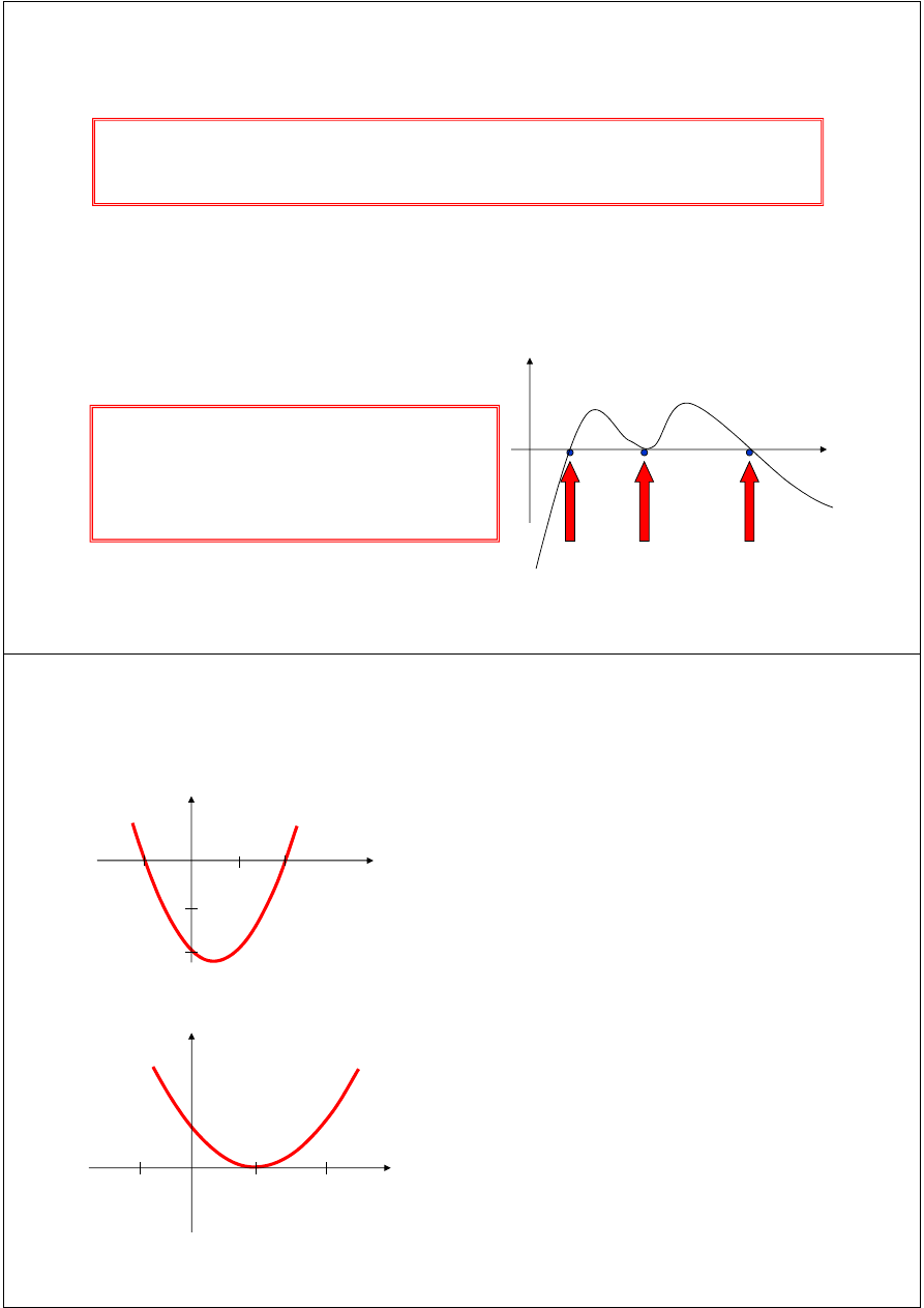
Graphical Interpretation of zeros:
real zeros of f(x)
f(x)
The real zeros of a function
f(x)
are
the values of
x
at which the graph of
the function crosses (or touches) the
x-axis
.
Simple / multiple zeros
(
)
)
1
at x
one
and
2
at x
(one
zeros
simple
two
has
2
2
)
1
(
)
(
2
−
=
=
−
−
=
−
+
=
x
x
x
x
x
f
(
)
)
2
(
1
)
(
−
+
=
x
x
x
f
( )
2
1
)
(
−
=
x
x
f
(
)
1
at x
2)
y
muliplicit
with
(zero
zeros
double
has
1
2
1
)
(
2
2
=
=
+
−
=
−
=
x
x
x
x
f

Multiple zeros
3
)
(
x
x
f
=
0
at
3
y
muliplicit
with
zero
a
has
)
(
3
=
=
=
x
x
x
f
0
at
3
y
muliplicit
with
zero
a
has
=
=
x
Any n
th
order polynomial has exactly n zeros (counting real and
complex zeros with their multiplicities).
Any polynomial with an odd order has at least one real zero.
If a function has a zero at x = r with multiplicity m then the
function and its first (m - 1) derivatives are zero at x = r and the m
th
derivative at r is not zero.
Roots of Equations & Zeros of Function
18
15
7
3
2
3
4
−
=
+
−
−
x
x
x
x
Given the equation:
Move all the terms to one side of the equation:
0
18
15
7
3
2
3
4
=
+
+
−
−
x
x
x
x
The zeros of f(x) are the same as the roots of the equation f(x) = 0
(which are -2, 3, 3 and -1.)
Define f(x) as:
( )
18
15
7
3
2
3
4
+
+
−
−
=
x
x
x
x
x
f

Solution methods
Several ways to solve nonlinear equations are possible:
Analytical Solutions
Possible for special equations only
Graphical Solutions
Graphical Solutions
Useful for providing initial guesses for other methods
Numerical Solutions
Open methods
Bracketing methods
Analytical methods
Analytical solutions are available for special equations only.
Analytical solution of :
0
2
=
+
+
c
x
b
x
a
b
roots
∆
±
−
=
ac
b
4
2
−
=
∆
No analytical solution is available for, e.g.:
0
=
−
−
x
e
x
a
roots
2
=
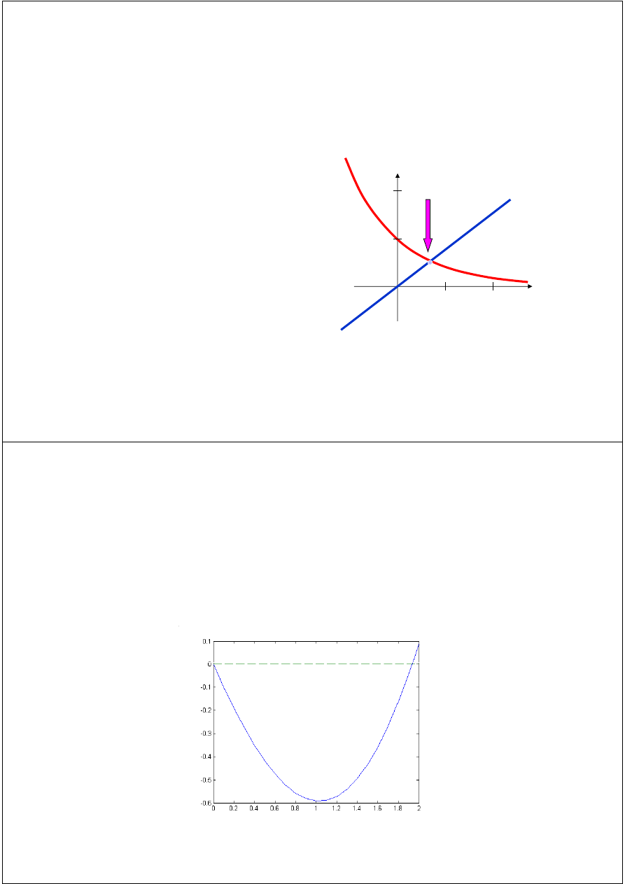
Graphical (‘starting’) methods
Graphical methods are useful to provide an initial guess
to be used by other methods.
solve
=
−
x
e
x
x
e
−
x
root
2
0.6
root
]
1
,
0
[
root
the
≈
∈
x
1 2
1
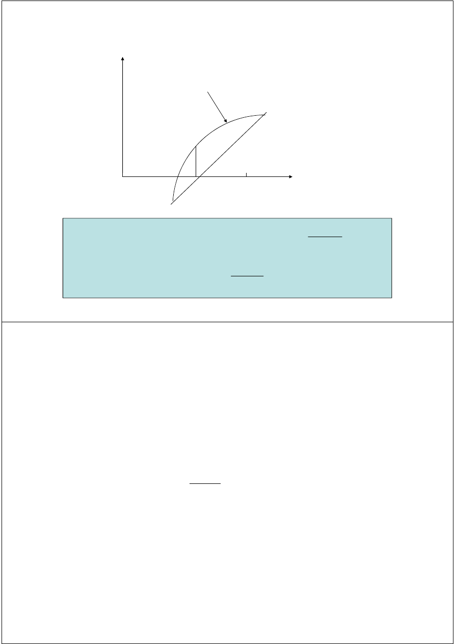
Graphical ‘starting’ methods
Initial approximation of roots of equation f(x) = 0 can be obtained by
plotting function f(x).
E.g. on the basis of Fig. 1 we know that the root of the considered
equation belongs to the band .
Fig. 1. Function and its roots.

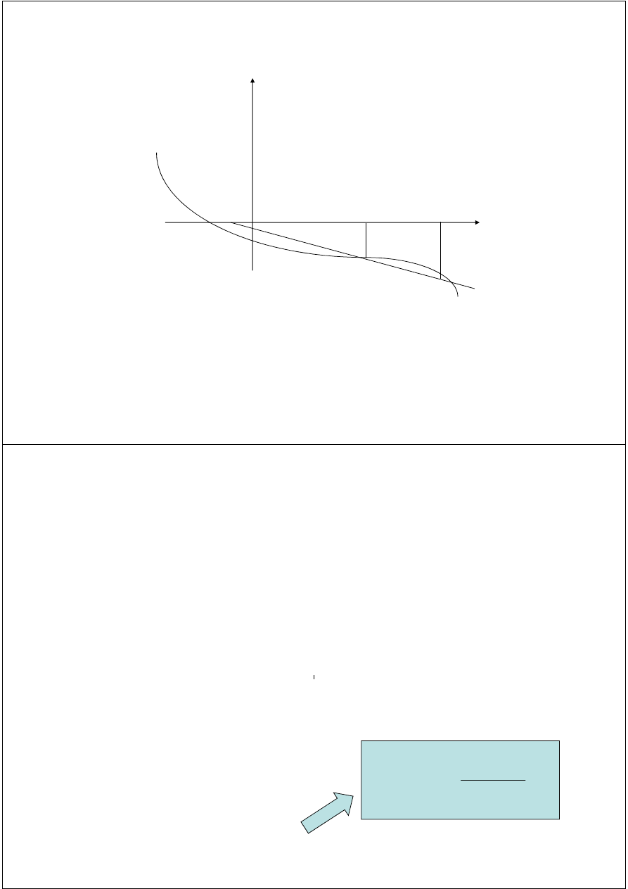
Graphical ‘starting’ methods
For the purposes of initial assessment of equation roots, we can
prepare table of values of function f(x).
x
(0,5)x
2
sinx
f(x)
1,6
0,64
-0,9996
< 0
1,8
0,81
-0,974
< 0
2,0
1,00
0,909
> 0
In general, if f(x) is continuous in the band (a, b) and f(a)f(b) < 0
then equation f(x) = 0 has at least one real root in the band (a, b).
Numerical methods
Many methods are available to solve nonlinear equations:
Bisection Method
Newton’s Method
Secant Method
Secant Method
False position Method
Muller’s Method
Bairstow’s Method
Fixed point iterations
……….

Bracketing methods
In bracketing methods, the method starts with an
interval that contains the root and a procedure is used to
obtain a smaller interval containing the root.
Examples of bracketing methods:
Examples of bracketing methods:
Bisection method
False position method
Open methods
In the open methods, the method starts with one or more
initial guess points. In each iteration, a new guess of the
root is obtained.
Open methods are usually more efficient than bracketing
methods.
methods.
They may not converge to a root.

BISECTION METHOD
BISECTION METHOD
Bisection method
Bisection method is one of the simplest and most reliable
methods of finding solution of nonlinear equations.
It belongs to the class of iterative methods, which means
that computations are repeated as long as the accuracy
criterion is not met.
criterion is not met.
The method requires estimation of band containing the
function root. If the function is continues and has a single
root in a given band, this condition is satisfied if function
values at the edges of a considered band have different
signs.
Slow convergence is the main method disadvantage.
Intermediate value theorem
Let f(x) be defined on the interval
[a, b].
Intermediate value theorem:
if a function is
continuous
and f(a)
a
b
f(a)
f(b)
if a function is
continuous
and f(a)
and f(b) have
different signs
then
the function has at least one zero
in the interval [a, b].
f(b)
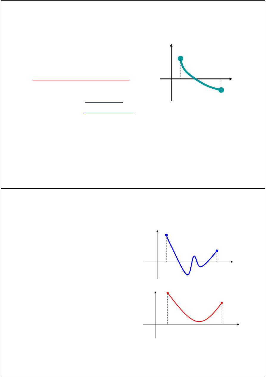
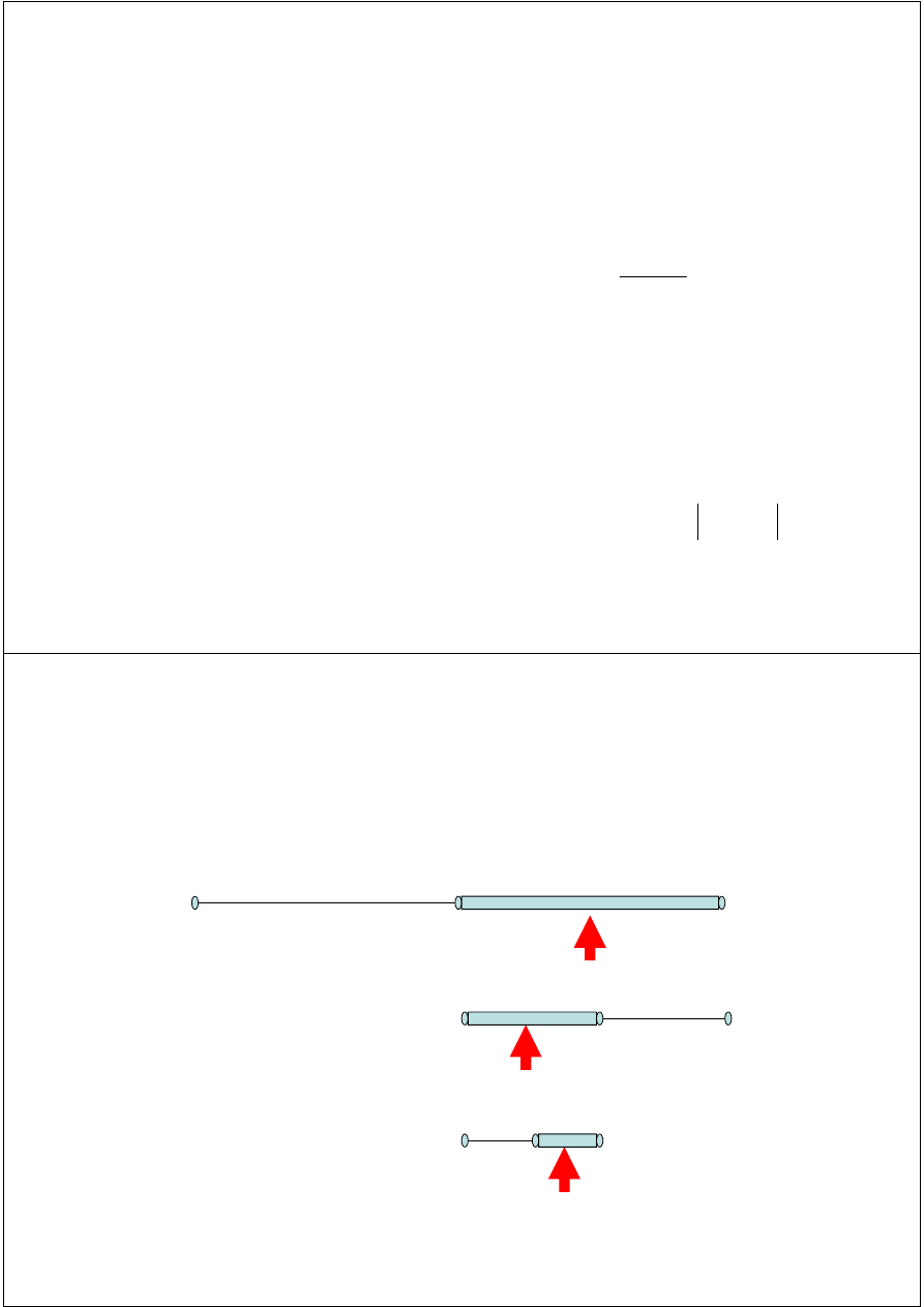
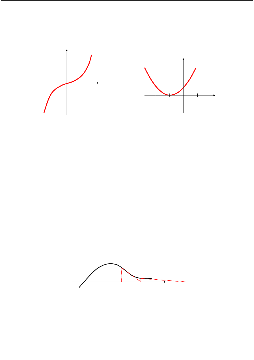
Examples
If f(a) and f(b) have the
same sign, the function may
have an even number of
real zeros or no real zeros in
a
b
The function has four
the interval [a, b].
Bisection method can not
be used in these cases.
a
b
The function has four
real zeros
The function has no real
zeros
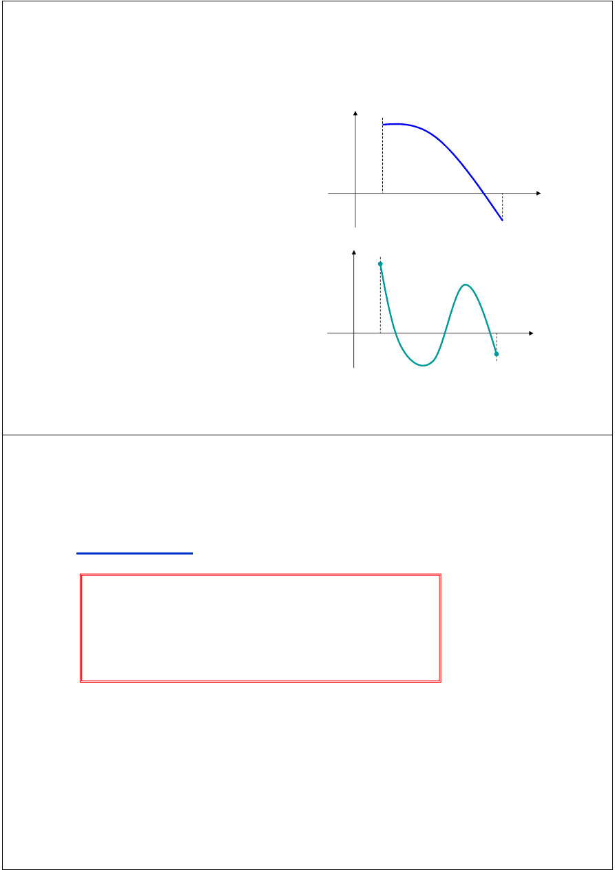
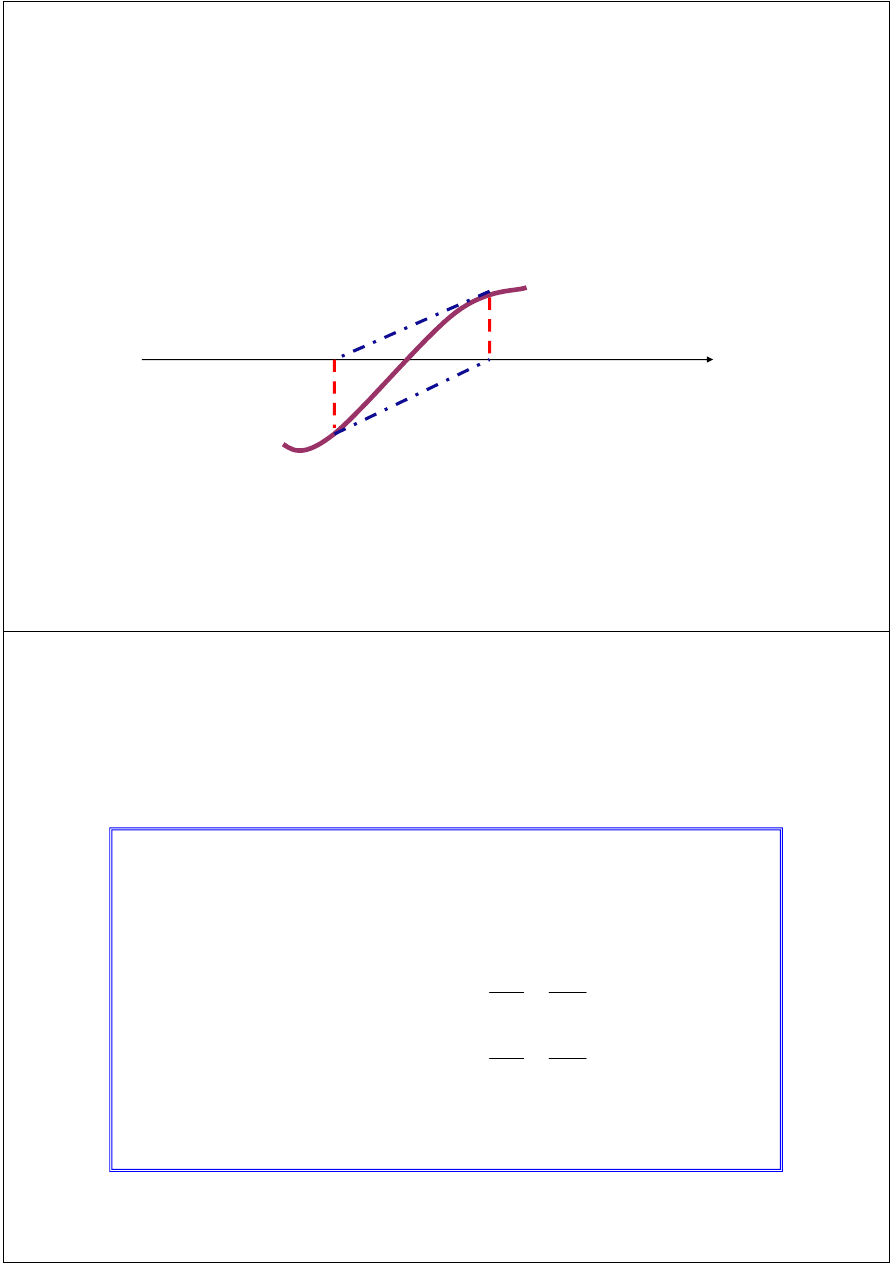
Examples
a
b
If
f(a)
and
f(b)
have
different
signs,
the
function has at least one
real zero.
a
b
real zero.
Bisection method can be
used to find one of the
zeros.
The function has one real
zero
The function has three real
zeros
Bisection Method
Assumptions:
Given an interval
[a, b]
f(x)
is continuous on
[a, b]
f(a)
and
f(b)
have opposite signs.
f(a)
and
f(b)
have opposite signs.
These assumptions ensure the existence of at least one
zero in the interval
[a, b]
and the bisection method
can be used to obtain a smaller interval that contains
the zero.
Algorithm of bisection method
Having band edges: a
i
< b
i
check the condition of sign change:
If the signs are different, determine point
and value of
the considered function f(c
i
) at this point.
( ) ( )
0
<
i
i
b
f
a
f
2
i
i
i
b
a
c
+
=
Decide which of the edge points should be replaced by the point c
i
.
Use the following criterion: if
then
otherwise
.
Repeat the above steps as long as the band being narrowed is
smaller than the assumed tolerance ε, which means that
.
( ) ( )
0
<
i
i
c
f
a
f
i
i
i
i
c
b
a
a
=
=
+
+
1
1
,
i
i
i
i
b
b
c
a
=
=
+
+
1
1
,
ε
≤
−
i
i
a
b
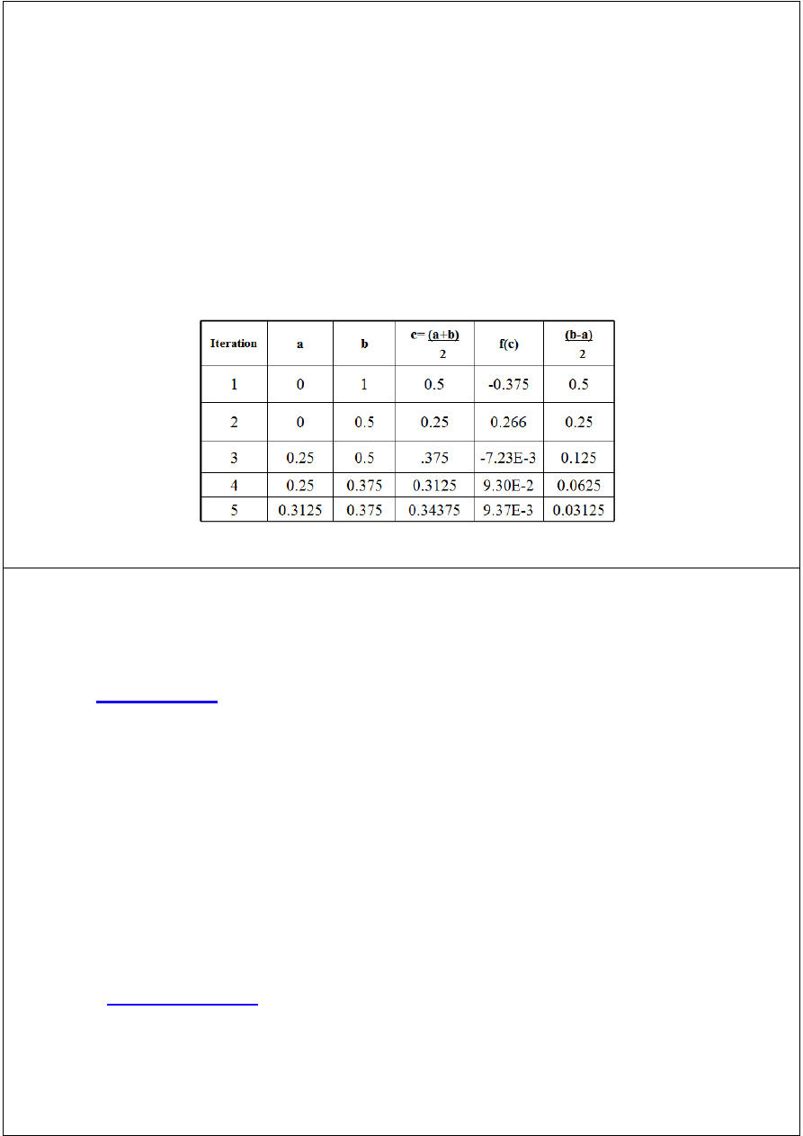
Example
+ + -
+ -
-
+ -
-
+ + -
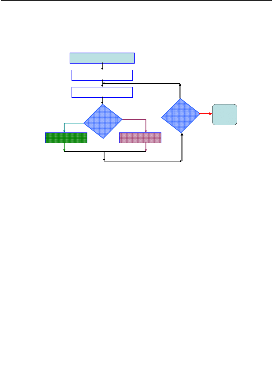
Flow Chart of Bisection Method
Start: given a, b and ε
u = f(a) ; v = f(b)
c = (a+b) /2 ; w = f(c)
no
is
u w <0
a=c; u= w
b=c; v= w
is
(b-a) /2<
ε
yes
yes
no
Stop
no
Example
Answer:
[0,2]?
interval
in the
1
3
)
(
:
of
zero
a
find
to
method
Bisection
use
you
Can
3
+
−
=
x
x
x
f
Answer:
( ) ( ) ( ) ( )
used
be
not
can
method
Bisection
satisfied
not
are
s
Assumption
0
3
3
1
2
0
and
2]
[0,
on
continuous
is
)
(
⇒
⇒
>
=
⋅
=
⋅
f
f
x
f

Example
Answer:
[0,1]?
interval
in the
1
3
)
(
:
of
zero
a
find
to
method
Bisection
use
you
Can
3
+
−
=
x
x
x
f
Answer:
( ) ( ) ( )( )
used
be
can
method
Bisection
satisfied
are
s
Assumption
0
1
1
1
1
0
and
[0,1]
on
continuous
is
)
(
⇒
⇒
<
−
=
=
-
*f
f
x
f
Stopping Criteria
Two common stopping criteria
1. Stop after a fixed number of iterations
2. Stop when the absolute error is less than a specified
value
How are these criteria related?

Though the root lies in a small interval, |f(x)| may not be
small if f(x) has a large slope.
Conversely if |f(x)| small, x may not be close to the root
if f(x) has a small slope.
So, we use both these facts for the termination criterion.
So, we use both these facts for the termination criterion.
We first choose an error tolerance on f(x): |f(x)| <
∈
and
m the maximum number of iterations.
Number of Iterations and Error Tolerance
Length of the interval (where the root lies) after n
iterations
We can fix the number of iterations so that the root lies
n
n
x
x
e
2
0
1
−
=
We can fix the number of iterations so that the root lies
within an interval of chosen length
∈
(error tolerance).
2
log
log
)
log(
0
1
∈
−
−
≥
⇒
≤∈
x
x
n
e
n
If n satisfies this, root lies within a distance of
ε
/2 of the
actual root.

Number of Iterations and Error Tolerance
−
=
≥
ε
a
b
n
log
error
desired
interval
initial
of
width
log
)
2
log(
)
log(
)
log(
ε
−
−
≥
a
b
n
ε
error
desired
11
9658
.
10
)
2
log(
)
0005
.
0
log(
)
1
log(
)
2
log(
)
log(
)
log(
?
e
:
such that
needed
are
iterations
many
How
0005
.
0
,
7
,
6
n
≥
⇒
=
−
=
−
−
≥
≤
=
=
=
n
a
b
n
b
a
ε
ε
ε
Example:
Example
use Bisection method to find a root of the equation
x = cos(x) with absolute error <0.02
assume the initial interval [0.5, 0.9]
Question 1: What is f (x) ?
Question 1: What is f (x) ?
Question 2: Are the assumptions satisfied ?
Question 3: How many iterations are needed ?
Question 4: How to compute the new estimate ?
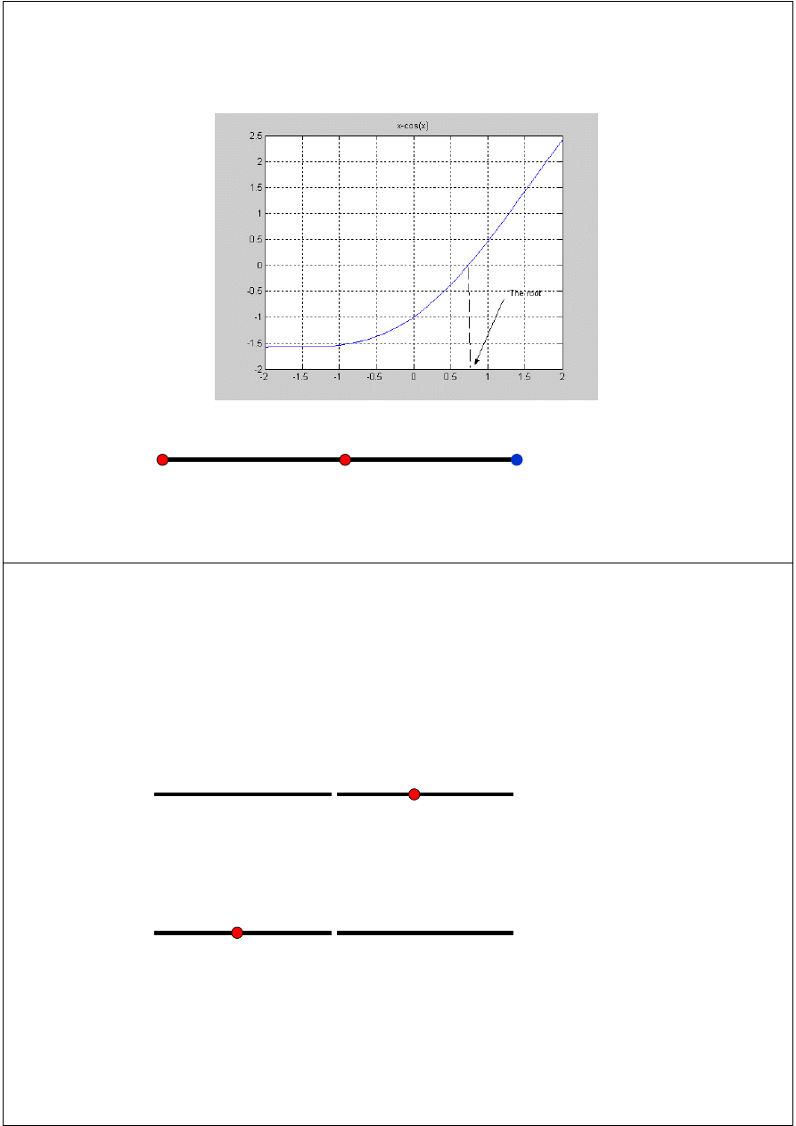
Example
f(a)=-0.3776
f(b) =
0.2784
a =0.5
c= 0.7
b= 0.9
Error < 0.2
Bisection Method
0.5 0.7 0.9
-0.3776 -0.0648
0.2784
Error < 0.1
0.7 0.8 0.9
-0.0648
0.1033 0.2784
Error < 0.05

Bisection Method
Error < 0.025
0.7 0.75 0.8
-0.0648
0.0183 0.1033
0.70 0.725 0.75
-0.0648 -0.0235
0.0183
Error < .0125
0.70 0.725 0.75
Initial interval containing the root: [0.5,0.9]
After 5 iterations:
Interval containing the root: [0.725, 0.75]
Best estimate of the root is 0.7375
| Error | < 0.0125
A Matlab Program of Bisection Method
a=.5; b=.9;
u=a-cos(a);
v=b-cos(b);
for i=1:5
c=(a+b)/2
fc=c-cos(c)
c =
0.7000
fc =
-0.0648
c =
0.8000
fc =
fc=c-cos(c)
if u*fc<0
b=c ; v=fc;
else
a=c; u=fc;
end
end
fc =
0.1033
c =
0.7500
fc =
0.0183
c =
0.7250
fc =
-0.0235
Example
Find the root of:
( )
( )
root
the
find
to
used
be
can
method
Bisection
0
)
(
)
(
1
)
1
(
,
1
0
*
continuous
is
*
[0,1]
:
interval
in the
1
3
)
(
3
⇒
<
⇒
−
=
=
+
−
=
b
f
a
f
f
f
x
f
x
x
x
f
root
the
find
to
used
be
can
method
Bisection
⇒
Bisection Method
Advantages
Simple
and easy to implement
One
function evaluation per iteration
The
size
of the interval containing the zero is reduced by
50% after each iteration
The
number of iterations
can be determined
a priori
The
number of iterations
can be determined
a priori
No
knowledge of the
derivative
is needed
The function does
not
have to be
differentiable
Disadvantage
Slow
to convergence

False Position Method
(Regula Falsi)
(Regula Falsi)
False Position Method (Regula Falsi)
Instead of bisecting the interval [x
0
, x
1
], we
choose the point where the straight line through
the end points meet the x-axis as x
2
and bracket
the root with [x
0
, x
2
] or [x
2
, x
1
] depending on the
the root with [x
0
, x
2
] or [x
2
, x
1
] depending on the
sign of f(x
2
).
False Position Method
(x
1
, f
1
)
(x
2
, f
2
)
y = f(x)
y
x
0
(x
0
, f
0
)
x
2
x
1
x
Straight line through (x
0
, f
0
), (x
1
, f
1
):
New end point x
2
:
)
(
1
0
1
0
1
1
x
x
x
x
f
f
f
y
−
−
−
+
=
1
0
1
0
1
1
2
f
f
f
x
x
x
x
−
−
−
=
False Position Method (Pseudo Code)
( )
0
1
x
f
f
,
=
−
−
=
f
x
x
x
x
1. Choose
∈
> 0 (tolerance on |f(x)| )
m > 0 (maximum number of iterations )
k = 1 (iteration count)
x
0
, x
1
(so that f
0
, f
1
< 0)
2. {
a) Compute
( )
2
2
1
0
1
0
1
1
2
x
f
f
,
=
−
−
=
f
f
f
x
x
3. While (|f
2
|
≥
∈
) and (k
≤
m)
a) Compute
b) If f
0
f
2
< 0 set x
1
= x
2
, f
0
= f
2
c) k = k+1
}
4. x = x
2
, the root.

Newton-Raphson Method /
Newton’s Method
Newton-Raphson Method / Newton’s Method
At an approximate x
k
to the root, the curve is
approximated by the tangent to the curve at x
k
and the next
approximation x
k+1
is the point where the tangent meets
the x-axis.
y
y = f(x)
root
x
0
x
x
1
x
2
ξ

Newton-Raphson Method / Newton’s Method
Newton’s method or the method of tangents (dedicated to
estimation of roots of nonlinear equations) is one of most popular
and efficient numerical methods.
As the main method disadvantages the requirement of function
derivative knowledge and method sensitivity to accuracy of root
derivative knowledge and method sensitivity to accuracy of root
initial values are treated.
In order to start a procedure realizing the Newton’s method it is
necessary to specify one starting point.
Tangent at (x
k
, f
k
):
This tangent cuts the x-axis at x
k+1
Newton-Raphson Method / Newton’s Method
( )
( )( )
k
k
k
x-x
x
f ´
x
f
y
+
=
)
(
)
(
1
k
k
k
k
x
f
x
f
x
x
′
−
=
+
Warning: If f´(x
k
) is very small, method fails.
Two function evaluations per iteration.
This tangent cuts the x-axis at x
k+1

Newton’s method algorithm
Compute value of function f(x
i
) and its derivative f ’(x
i
) in the
current point x
i
.
Plot tangent to a considered function in point (x
0
, f(x
0
)) and
determine the point in which this tangent crosses Ox axis. Use
equation: .
( )
x
f
Assume point x
i
+1 as a consecutive root approximation.
As a ‘stop’ criterion assume obtaining consecutive approximations
differing from each other less than assumed accuracy together with
a small value of function:
( )
( )
i
i
i
i
x
f
x
f
x
x
'
1
−
=
+
ε
≤
−
+
i
i
x
x
1
( )
ε
≤
n
x
f
Newton’s Method - Pseudo code
1. Choose
∈
> 0
(function tolerance |f(x)| <
∈
)
m > 0
(Maximum number of iterations)
x
0
(initial approximation)
k
(iteration count)
Compute f(x
0
)
2. Do { q = f
′
(x )
(evaluate derivative at x )
2. Do { q = f
′
(x
0
)
(evaluate derivative at x
0
)
x
1
= x
0
- f
0
/ q
x
0
= x
1
f
0
= f(x
0
)
k = k+1 }
3. While (|f
0
|
≥
∈
) and (k
≤
m)
4. x = x
1
the root.

Newton’s Method for finding the square
root of a number
k
k
k
k
x
a
x
x
x
2
2
2
1
−
−
=
+
( )
0
a
-
x
x
f
2
2
=
=
Example: a = 5, initial approximation x
0
= 2.
x
1
= 2,25
x
2
= 2,236111111
x
3
= 2,236067978
x
4
= 2,236067978
Example
9
)
(
3
33
33
4
)
(
'
)
(
:
1
Iteration
1
4
3
'
4
,
3
2
function
the
of
zero
a
Find
0
0
0
1
2
0
2
3
=
−
=
−
=
+
−
=
=
−
+
−
=
x
f
x
f
x
f
x
x
x
x
(x)
f
x
x
x
x
f(x)
2130
.
2
0742
.
9
0369
.
2
4375
.
2
)
(
'
)
(
:
3
Iteration
4375
.
2
16
9
3
)
(
'
)
(
:
2
Iteration
2
2
2
3
1
1
1
2
=
−
=
−
=
=
−
=
−
=
x
f
x
f
x
x
x
f
x
f
x
x

Example
k
(Iteration)
x
k
f(x
k
)
f’(x
k
)
x
k+1
|x
k+1
–x
k
|
0
4
33
33
3
1
1
3
9
16
2.4375
0.5625
1
3
9
16
2.4375
0.5625
2
2.4375
2.0369
9.0742
2.2130
0.2245
3
2.2130
0.2564
6.8404
2.1756
0.0384
4
2.1756
0.0065
6.4969
2.1746
0.0010
Convergence Analysis
such that
0
exists
then there
0
'
.
0
where
r
at x
continuous
be
'
'
'
,
Let
:
Theorem
1
C
-r
x
-r
x
(r)
f
If
f(r)
(x)
f
(x) and
f
f(x)
k
δ
δ
+
≤
⇒
≤
>
≠
=
≈
)
(
'
min
)
(
'
'
max
2
1
such that
0
0
2
1
0
x
f
x
f
C
C
-r
x
-r
x
-r
x
-r
x
k
k
δ
δ
δ
≤
≤
+
=
≤
⇒
≤

Convergence Analysis - remarks
When the guess is close enough to a
simple
root of
the function then Newton’s method is guaranteed to
converge quadratically.
Quadratic convergence means that the number of
correct digits is nearly doubled at each iteration.
Problems with Newton’s Method
If the initial guess of the root is far from the
root the method may not converge.
Newton’s method converges linearly near
multiple zeros { f(r) = f’(r) =0 }. In such a case,
modified algorithms can be used to regain the
quadratic convergence.
Multiple Roots
(
)
2
1
)
(
+
=
x
x
f
3
)
(
x
x
f
=
1
at
zeros
0
at x
zeros
two
has
three
has
-
x
f(x)
f(x)
=
=
Problems with Newton’s Method
- Runaway -
The estimates of the root is going away from the root.
x
0
x
1
Problems with Newton’s Method
- Cycle -
x = x = x
The algorithm cycles between two values x
0
and x
1
x
0
= x
2
= x
4
x
1
= x
3
= x
5
Newton’s Method for Systems of Non Linear
Equations
[
]
−
=
=
−
+
1
1
0
)
(
)
(
'
'
0
)
(
of
root
the
of
guess
initial
an
:
X
F
X
F
X
X
Iteration
s
Newton
x
F
X
Given
k
k
k
k
[
]
∂
∂
∂
∂
∂
∂
∂
∂
=
=
−
=
+
M
M
M
2
2
1
2
2
1
1
1
2
1
2
2
1
1
1
)
(
'
,
,...)
,
(
,...)
,
(
)
(
)
(
)
(
'
x
f
x
f
x
f
x
f
X
F
x
x
f
x
x
f
X
F
X
F
X
F
X
X
k
k
k
k

Example
• Solve the following system of equations:
0
,
1
guess
Initial
0
5
0
5
0
2
2
=
=
=
−
−
=
−
−
+
y
x
y
xy
x
x
.
x
y
0
,
1
guess
Initial
=
=
y
x
=
−
−
−
−
=
−
−
−
−
+
=
0
1
,
1
5
5
2
1
1
2
'
,
5
5
0
0
2
2
X
x
y
x
x
F
y
xy
x
x
.
x
y
F
Solution Using Newton’s Method
=
−
−
−
=
−
=
−
−
−
−
=
=
−
=
−
−
−
−
+
=
−
25
.
0
25
.
1
1
5
0
6
2
1
1
0
1
6
2
1
1
1
5
5
2
1
1
2
'
,
1
5
0
5
5
0
:
1
Iteration
1
1
2
2
.
X
x
y
x
x
F
.
y
xy
x
x
.
x
y
F
=
−
−
=
−
=
=
=
−
−
2126
.
0
2332
.
1
0.25
-
0.0625
25
.
7
25
.
1
1
1.5
25
.
0
25
.
1
25
.
7
25
.
1
1
1.5
'
,
0.25
-
0.0625
:
2
Iteration
25
.
0
1
6
2
0
1
2
X
F
F

Example
Try this
• Solve the following system of equations:
0
2
0
1
2
2
2
=
−
−
=
−
−
+
y
y
x
x
x
y
0
,
0
guess
Initial
=
=
y
x
=
−
−
−
=
−
−
−
−
+
=
0
0
,
1
4
2
1
1
2
'
,
2
1
0
2
2
2
X
y
x
x
F
y
y
x
x
x
y
F
Example - Solution
−
−
−
−
−
0.1980
0.5257
0.1980
0.5257
0.1969
0.5287
2
.
0
6
.
0
0
1
0
0
_
__________
__________
__________
__________
__________
__________
5
4
3
2
1
0
k
X
Iteration

The Secant Method
The Secant Method
The Secant Method
The Newton’s Method requires 2 function evaluations (f, f’).
The Secant Method requires only 1 function evaluation and
converges as fast as Newton’s Method at a simple root.
Start with two points x , x
near the root (no need for
Start with two points x
0
, x
1
near the root (no need for
bracketing the root as in Bisection Method or Regula Falsi
Method).
x
k-1
is dropped once x
k+1
is obtained.
The Secant Method (Geometrical Construction)
y = f(x
1
)
x
2
x
0
x
y
x
1
Two initial points x
0
, x
1
are chosen.
The next approximation x
2
is the point where the straight line
joining (x
0
, f
0
) and (x
1
, f
1
) meet the x-axis.
Take (x
1
, x
2
) and repeat.
ξξξξ
(x
0
, f
0
)
(x
1
,f
1
)
x
The Secant Method (Pseudo Code)
1. Choose
∈
> 0 (function tolerance |f(x)|
≤
∈
)
m > 0 (Maximum number of iterations)
x
0
, x
1
(Two initial points near the root )
f
0
= f(x
0
)
f
1
= f(x
1
)
k = 1 (iteration count)
k = 1 (iteration count)
2. Do {
x
0
= x
1
f
0
= f
1
x
1
= x
2
f
1
= f(x
2
)
k = k+1 }
3. While (|f
1
|
≥
∈
) and (m
≤
k)
f
f
f
x
x
x
x
−
−
−
=
0
1
2
1
1
2

Convergence notation
N
n
x
x
N
x
x
x
x
n
n
>
∀
<
−
>
ε
ε
:
that
such
exists
there
0
every
to
if
to
to
said
is
,...
,...,
,
sequence
A
2
1
converge
Convergence notation
C
x
x
C
x
x
x
x
x
x
x
n
n
n
≤
−
≤
−
−
+
+
1
1
2
1
:
e
Convergenc
Quadratic
:
e
Convergenc
Linear
.
to
converge
,....,
,
Let
C
x
x
x
x
P
C
x
x
p
n
n
n
n
≤
−
−
≤
−
+
+
1
2
1
:
order
of
e
Convergenc
:
e
Convergenc
Quadratic

Speed of convergence
We can compare different methods in terms of their
convergence rate.
Quadratic convergence
is faster than
linear convergence
.
A method with convergence order q converges faster
than a method with convergence order p if q > p.
than a method with convergence order p if q > p.
Methods of convergence order p > 1 are said to have
super linear convergence
.
Order of Convergence
Bisection method p = 1 ( linear convergence )
False position - generally Super linear ( 1 < p < 2 )
5
1
+
Secant method (super linear)
Newton - Raphson method p = 2 quadratic
618
,
1
2
5
1
=
+

Remarks on convergence
The
False Position
method in general converges faster than
the
Bisection
method (but not always).
The
Bisection
method and the
False Position
method are
guaranteed for convergence.
The
Secant
method and the
Newton-Raphson
method are
not guaranteed for convergence.
Comparison of Root
Finding Methods
Advantages/disadvantages
Examples

Summary
Method Pros
Cons
Bisection
- Easy, Reliable, Convergent
- One function evaluation per
iteration
- No knowledge of derivative is
needed
- Slow
- Needs an interval [a,b]
containing the root, i.e.,
f(a)f(b)<0
needed
Newton
- Fast (if near the root)
- Two function evaluations per
iteration
- May diverge
- Needs derivative and an
initial guess x
0
such that
f’(x
0
) is nonzero
Secant
- Fast (slower than Newton)
- One function evaluation per
iteration
- No knowledge of derivative is
needed
- May diverge
- Needs two initial points
guess x
0
, x
1
such that
f(x
0
)- f(x
1
) is nonzero
Example
In estimating the root of: x - cos(x) = 0, to get more
than 13 correct digits:
4
iterations of Newton
(x
0
=0.8)
4
iterations of Newton
(x
0
=0.8)
43
iterations of Bisection method (initial interval
[0.6, 0.8])
5
iterations of Secant method
( x
0
=0.6, x
1
=0.8)

To sum up …
Roots of nonlinear equations usually:
can’t be described by closed-form formulas,
or these formulas are too complicated to be used in practice.
Therefore methods of solving nonlinear equation are based on
the idea of consecutive approximations or linearization.
the idea of consecutive approximations or linearization.
These methods require one (or more) root initial values and
return the sequence x
0
, x
1
, x
2
, … that is likely to converge to the
real value.
In some cases, in order to obtain convergence, it is sufficient to
know band <a, b> containing a root.
To sum up …
Other methods require initial approximation that is close enough to
the considered root (these methods usually converge more quickly
than remaining methods).
Therefore the nonlinear equations are usually solved in two steps:
first the root (or a band containing the root) is roughly evaluated, next
first the root (or a band containing the root) is roughly evaluated, next
more accurate solution is estimated.

Lecture prepared on the basis of:
Avudainayagam A.: Course CS-110: Computational
Engineering Part 3,
http://www.cs.iitm.ernet.in/~swamy/num_methods.ppt
Fortuna Z., Macukow B., Wąsowski J.: Metody
numeryczne, WNT, Warszawa, 1982.
Thank you for your attention!
Wyszukiwarka
Podobne podstrony:
2 Sieci komputerowe 09 03 2013 [tryb zgodności]
3 Sieci komputerowe 23 03 2013 [tryb zgodności]
Dzia alno kredytowa 2013 [tryb zgodno ci]
ZPiU prezentacja I 2013 [tryb zgodności]
dp 651 wykl miazdzyca-bez rycin wl 2013 [tryb zgodnosci](czyli 2014.03.04)
czas pracy grudzień 2013 [tryb zgodności]
Introduction to Literature 1 2013 tryb zgodnosci
elementy reologii 2013 tryb zgodnosci
2 Sieci komputerowe 09 03 2013 [tryb zgodności]
3 Sieci komputerowe 23 03 2013 [tryb zgodności]
więcej podobnych podstron