[Форекс] The Cost of Technical Trading Rules in the Forex Market

The Cost of Technical Trading Rules in the Forex Market:

A Utility-based Evaluation

Hans Dewachter and Marco Lyrio

ERIM R

EPORT

ERIES

ESEARCH IN

ANAGEMENT

ERIM Report Series reference number

ERS-2003-052-F&A

Publication status / version

May 2003

Number of pages

Email address corresponding author

hdewachter@fbk.eur.nl

Address

Erasmus Research Institute of Management (ERIM)
Rotterdam School of Management / Faculteit Bedrijfskunde

Rotterdam School of Economics / Faculteit Economische

Wetenschappen

Erasmus Universiteit Rotterdam
PoBox 1738
3000 DR Rotterdam, The Netherlands
Phone:

# 31-(0) 10-408 1182

Fax:

# 31-(0) 10-408 9640

Email:

info@erim.eur.nl

Internet:

www.erim.eur.nl

Bibliographic data and classifications of all the ERIM reports are also available on the ERIM website:

www.erim.eur.nl

ERASMUS RESEARCH INSTITUTE OF MANAGEMENT

REPORT SERIES

RESEARCH IN MANAGEMENT

IBLIOGRAPHIC DATA AND CLASSIFICATIONS

Abstract

We compute the opportunity cost for rational risk averse agents of using technical trading rules in
the foreign exchange rate market. Our purpose is to investigate whether these rules can be
interpreted as near-rational investment strategies for rational investors. We analyze four di.erent
exchange rates and find that the opportunity cost of using chartist rules tends to be prohibitively
high. We also present a method to decompose this opportunity cost into parts related to investor’s
irrationality and misallocation of wealth. The results show that irrationality of chartist beliefs is an
important component of the total opportunity cost of using technical trading rules.

5001-6182 Business

5601-5689
4001-4280.7

Accountancy, Bookkeeping
Finance Management, Business Finance, Corporation Finance

Library of Congress
Classification
(LCC)

HG 4638

Technical analysis securities

Business Administration and Business Economics

M 41
G 3

Accounting
Corporate Finance and Governance

Journal of Economic
Literature
(JEL)

F 31
G 15

Foreign Exchange
International Financial Markets

85 A

Business General

225 A
220 A

Accounting General
Financial Management

European Business Schools
Library Group
(EBSLG)

220 T

Quantitative methods for financial methods

Gemeenschappelijke Onderwerpsontsluiting (GOO)

85.00

Bedrijfskunde, Organisatiekunde: algemeen

85.25
85.30

Accounting
Financieel management, financiering

Classification GOO

85.33

Beleggingen

Bedrijfskunde / Bedrijfseconomie

Accountancy, financieel management, bedrijfsfinanciering, besliskunde

Keywords GOO

Effectenhandel, Beleggingen, wisselkoersen, Rationaliteit

Free keywords

technical trading rule, exchange rate

The Cost of Technical Trading Rules in the Forex Market:

A Utility-based Evaluation

Hans Dewachter

a,b∗

and Marco Lyrio

CES, Catholic University of Leuven

RIFM and ERIM, Erasmus University Rotterdam

May 2003

Abstract

We compute the opportunity cost for rational risk averse agents of using technical trading
rules in the foreign exchange rate market. Our purpose is to investigate whether these rules
can be interpreted as near-rational investment strategies for rational investors. We analyze
four diﬀerent exchange rates and find that the opportunity cost of using chartist rules tends
to be prohibitively high. We also present a method to decompose this opportunity cost
into parts related to investor’s irrationality and misallocation of wealth. The results show
that irrationality of chartist beliefs is an important component of the total opportunity
cost of using technical trading rules.

Keywords:

technical trading rule, exchange rate.

J.E.L.:

F31, G15.

∗

Corresponding author. Address: Center for Economic Studies, Catholic University of Leuven, Naamses-

traat 69, 3000 Leuven, Belgium. Tel: (+)32(0)16-326859, e-mail: hans.dewachter@econ.kuleuven.ac.be. We are
grateful for financial support from the FWO-Vlaanderen (Project No.:G.0332.01). The latest version of this pa-
per can be downloaded from http://www.econ.kuleuven.ac.be/ew/academic/intecon/Dewachter/default.htm.
The authors are responsible for remaining errors.

Introduction

Despite the numerous studies reporting the pervasive use of technical trading rules and their

profitability,

there is still a considerable amount of scepticism in the academic literature

regarding their true value. Critics of chartist rules often point to the seemingly suboptimal

nature of the portfolio composition implied by these rules (e.g. Skouras, 2001). After all,

investment strategies based on technical trading rules (i) restrict the information set to a

narrow group of pre-defined information variables, (ii) assume a positive relation of the signal

with future expected excess returns

, and (iii) imply a bang-bang type of investment strategy,

i.e. a strategy where all wealth is invested either short or long. Each of these assumptions

goes against the standard rational investor paradigm. The first two assumptions possibly go

against the rationality of expectations formation, while the third is in general at odds with

the assumption of risk aversion.

In this paper, we assess the value of technical trading rules for rational risk averse investors.

The main motivation being that even if technical trading rules turn out to be suboptimal

rules, the observed practice of using these rules could still be near rational for a large class

of risk averse agents. More specifically, if the cost (as measured, for instance, by certainty

equivalents) for risk averse agents of using technical trading rules is low, one may argue that

following these (irrational) rules of thumb may come close to the optimal trading strategy

and could, therefore, be rationalized in terms of information cost type of arguments.

The opportunity cost associated with the use of technical trading rules for risk averse

agents can be decomposed in two components: the first component relates to the potential

error in the assumed relation between the chartist signal and the expected future return (ex-

pectational error); the second component originates from the suboptimality of the investment

strategy (allocation error). We present a simple method to compute each of these components.

The method involves the introduction of a hypothetical risk neutral agent. Risk neutral liq-

uidity constrained agents have in common with technical traders that investment strategies

will be typically bang-bang solutions, i.e. either invest all wealth in the long or in the short

side. In fact, as argued by Skouras (2001), as long as the chartist signal is one-to-one with

the expected future excess return, chartist trading strategies are equivalent to those of a ra-

tional risk neutral liquidity constrained agent. In this case, chartist rules are, therefore, also

rational. Diﬀerences in the trading positions of a risk neutral and a technical trader isolate,

therefore, the costs associated with expectational errors in the relation between the technical

trading signal and the expected return. The second cost component -associated with the

misallocation of wealth- can be recovered by contrasting the portfolio positions of risk averse

and risk neutral agents. Since both agents have identical expectations, the diﬀerence in their

trading positions can be linked to the costs of risk averse agents investing according to bang-

bang investment strategies. Combining these cost components results in a total opportunity

See, among others, Gençay (1999); LeBaron (1992, 1999, 2000); Neely et al (1997); and Taylor (1980).

We assume here a standardized rule where a positive (negative) technical trading signal corresponds to a

long (short) investment position.

cost for a rational risk averse agent of using technical trading rules. We use this technique

to identify possible classes of risk averse agents for which these opportunity costs are limited.

In this case, one could perhaps rationalize the use of trading rules in terms of near-rational

behavior.

Computing the costs of chartist trading rules implies both the identification of technical

trading signals and the design of a statistical model to relate the conditional moments of the

excess returns to the technical trading signal. In this paper, we restrict the analysis to the

class of moving average signals, or rules. We select this class as it constitutes the most widely

used class of technical trading rules in the foreign exchange market. These rules have also

been shown to be robust in their profit generating capacities. We also opt for a relatively

simple model relating return moments to the trading signal. While more advanced techniques

such as the nonparametric regression technique of Brandt (1999), or nonlinear models such as

neural nets (Gençay, 1999) or Markov switching models (e.g. Dewachter, 2001) could be used,

we try to strike a balance between generality and computational costs. We, therefore, use a

regression approach to estimate possible time-varying parameters of a Taylor expansion of the

relation between return moments and trading signals. This approach is suﬃciently flexible

to allow for nonlinearities in the signal-return moment relation while at the same time it is

computationally tractable so as to allow for continuous updating of the parameters.

The remainder of the paper is organized in three main sections. In section 2, we discuss

the proposed decomposition of the costs associated with the use of technical trading rules.

The empirical results are presented in section 3. In this section, we first analyze the statistical

models relating trading signals to return moments. We do find evidence of a nonlinear relation

both for the expected return and for the conditional variance. Using these models to construct

the optimal portfolio rule for classes of risk averse agents, we subsequently analyze the value

of technical trading signals and the costs associated with following technical trading rule

strategies. We summarize the main findings of the paper in the concluding section.

The opportunity cost of technical trading rules

Technical trading rules are typically rules of thumb that relate a certain information variable,

the technical trading signal, to a trading position. Denoting the time t technical trading signal

by z

, the technical trading rule specifies a mapping from the signal z

to an advised trading

position ω

) . A typical feature is the discontinuity in the mapping ω

). We assume

that the trading signal has been standardized such that the trading rule, i.e. the mapping

from the signal to the trading position, can be described by:

) =











b if z

> 0

0 if z

= 0

−b if z

< 0

(1)

where b > 0 denotes the liquidity constraint faced by the chartist trader.

Obviously, the optimal portfolio composition in general diﬀers from the one implied by

the technical trading rule strategy. As noted by Skouras (2001), utility-based optimal trading

rules typically depend on various factors, including the risk aversion and rational expectations

about the conditional return distribution. For a rational, liquidity constrained, risk averse

agent, the optimal trading strategy can be written as the solution to the following standard

portfolio allocation problem:

max

[U (W

t+1

)]

s.t.
∆W

t+1

= W

(1 + r

+ ωX

t+1

)

ω ∈ [−b, b]

(2)

where r

denotes the risk-free interest rate, and X

t+1

the speculative return above the riskless

rate obtained from investing in the risky asset. Note, moreover, that we implicitly assume that

the expectations are adapted to the information set used to construct the technical trading

signal z

. Formally, we assume that E

t+1

] = E [X

t+1

| z

] . By assuming a second order

Taylor expansion, we recast the above problem into a standard mean variance problem with

optimal portfolio allocation:

∗

t+1

− r

]

γV ar

t+1

)

(3)

where γ denotes the investor’s level of relative risk aversion. Since typical technical trading

rules simply specify positions (long or short), only under very restrictive circumstances will

these technical trading rules emerge as optimal trading rules. This is only possible, as men-

tioned by Skouras (2001), in the case of risk neutrality combined with liquidity constraints.

In this case, the typical optimal portfolio is a bang-bang solution and the investment position

is determined based only on the sign of the expected return. More formally, for a risk neutral

investor (γ = 0), the optimal trading rule is given by:

∗











b if E

t+1

] > 0

0 if E

t+1

] = 0

−b if E

t+1

] < 0

(4)

A small remark to be made to the above mentioned Skouras (2001) result is, however, that even

this bang-bang solution under risk neutrality only collapses to the standard technical trading

rule if the relation between the expected return and the chartist signal is one-to-one. Making

this additional assumption we have that the optimal risk neutral trading rule under liquidity

constraints collapses to the chartist rule. More formally, only if the equivalences below hold

Although not considered here, trading rules can also include bands of inaction.

will the optimal rule be equivalent to the standard chartist trading rule (ω

∗

= ω

) as

presented in eq. (1):

t+1

] > 0 ⇔ z

> 0,

t+1

] = 0 ⇔ z

= 0, and

t+1

] < 0 ⇔ z

< 0.

(5)

Technical trading rules are, therefore, not necessarily irrational trading strategies. To the

extent that the information variable z

corresponds one-to-one with the rationally expected

direction of the return, the strategy is optimal for risk neutral agents. Moreover, given the

continuity of the portfolio positions in γ, technical trading strategies could also function as

near-rational trading rules for a specific subclass of risk averse agents, i.e. for γ s close to

zero. If the level of relative risk aversion is relatively high, so that optimal allocation diﬀers

substantially from the risk neutral case, or if the chartist trading signal is not one-to-one

with rational expected returns, could the opportunity cost of following a technical trading, Λ,

become prohibitively high. This cost can be quantified as the following certainty equivalent:

Λ(z) = (ω

∗

− ω

) E

t+1

− r] −

1
2

γ ω

∗ 2

− ω

V ar

t+1

) .

(6)

The expected cost of following the chartist trading rule ω

instead of the optimal strategy

can be decomposed in two separate eﬀects. A first eﬀect is due to the possible error in

expectations made by chartist beliefs. A second eﬀect relates to the suboptmality of the

actual portfolio position. In order to separate these eﬀects, we make use of the optimal

trading strategy of the risk neutral agent, ω

RN :

Λ(z) = Λ

EXP

(z) + Λ

ALL

(z)

EXP

(z) = (ω

∗

− ω

) E

t+1

− r

]

ALL

(z) = (ω

∗

− ω

) E

t+1

− r

] −

1
2

γ ω

∗ 2

− ω

V ar

t+1

) .

(7)

By construction, both cost components are nonnegative and have a clear interpretation in

terms of percentage certainty equivalents. The first term, Λ

EXP

(z), models the loss due to

the possible diﬀerences between the technical and rational expectations. To the extent that

the chartists beliefs are inconsistent with the rationally expected sign of the future returns,

following chartist trading rules results in a loss in expected terms. Also, if chartist beliefs with

respect to the direction are consistent with rational expectation forecasts of future returns, i.e.

the equivalence between z and E[X] holds, this expectations term drops out as risk neutral

and chartist trading strategies become the same, ω

= ω

. The second cost component,

ALL

(z), originates from the possible suboptimality of wealth allocation of the technical

trading rule. Since technical trading rules advice a bang-bang wealth allocation, i.e. either

Adding and subtracting ω

in the first term on the right-hand side and noting that independent of z,

2
RN

= ω

2
CH

almost surely, we obtain the proposed decomposition.

full long or short position -depending on the sign of z−, technical trading rules neglect the
riskiness of the trading position. Risk averse agents obviously take this into account in their

trading strategies. The cost to a rational risk averse agent of following the technical trading

rule can thus be computed in terms of the diﬀerences in the certainty equivalents. This

cost, as stated above, can be decomposed into a cost due to the irrationality in expectation

formation of the technical trading rule and due to the suboptimality of the wealth allocation.

Finally, averaging over the frequency of occurrence of each trading signal, one obtains the

unconditional certainty equivalence costs as well as its decomposition.

Empirical analysis

3.1

Data and technical trading rules

The empirical analysis is performed for a set of technical trading rules applied to the exchange

rates of four currencies against the U.S. dollar: the German mark, the British pound, the

Japanese yen, and the Swiss franc. Exchange rates are expressed in the standard way as the

price in the domestic currency of one U.S. dollar, considered here as the foreign currency. We

use daily data for the above spot exchange rates obtained from Datastream for the period

January 1, 1973 to March 25, 2003, yielding a total of 7886 exchange rate returns.

The type of a trading rule depends on the way the trading signal is computed. In this

paper, we restrict the empirical analysis to the class of moving average trading rules. This is

one of the most used types of trading rules since the early seventies and has shown to generate

excess profits through time in the foreign exchange market. Furthermore, it is the one that

seems to be robust also in out-of-sample analysis (see, for instance, Neely et al., 1997). Due

to its widespread use, this choice also aims at reducing possible selection bias with respect

to the chosen class of trading rules. The technical trading signal z

for this class of rules

is constructed as the diﬀerence between a short and a long moving average window of past

exchange rate returns:

S−1

j=0

∆e

t−j

−

L−1

j=0

∆e

t−j

(8)

where e

denotes the natural logarithm of the exchange rate at time t, and S(L) denotes

the size or number of observations of the short (long) window of the moving average signal.

∆e

t−j

= e

− e

t−1

expresses the exchange rate return at time t. The investment position at

each point in time is then determined based on the sign of z

, as expressed in eq. (1). We

consider three types of trading signals (or rules) depending on the number of days incorporated

in the short (S) and long (L) window of the moving average rule. The following trading rules

are used. Rule 1: S = 10, L = 50; Rule 2: S = 20, L = 100; and Rule 3: S = 40, L = 200.

Due to the backward-looking nature of the moving average signal, the eﬀective number of

data points in the sample of each trading rule depends on the size of the long window used

to compute the trading signal.

Finally, in the computation of the return from investing in the exchange rate market, we

disregard the interest rate diﬀerential between the countries.

Besides the fact that these

data are not readily available, LeBaron (1999) shows that the exclusion of the interest rate

diﬀerential is unimportant for trading rule results. We also adopt an arbitrary value for the

risk free interest rate equal to zero.

Table 1 presents the standard result found in the literature that investing according to

technical trading rules generate significant mean excess returns. In our case, in all but one

case mean excess returns are statistically significant at the 10% level, and in eight out of the

twelve cases at the 5% level. Note, however, that the trading rule profits are not homogeneous

across positive and negative signals. Typically, trading rules are profitable in one of the two

investment positions. For the British pound-U.S. dollar, and for the three rules considered,

only a positive signal results in significant excess returns. For the other three exchange rates,

the opposite occurs, with one exception where neither signals generate significant excess

returns.

Insert Table 1

3.2

Least squares prediction models

Central in the above analysis is the projection of expected future return moments on the

technical trading signal z

. Naturally, the type of model used to project these moments on

the set of chartist signals influences the results regarding the costs of using chartist strategies.

In this paper, we try to strike a balance between the generality in the class of functions used

to project moments and the computational cost of continuously updating these projections

to take into account the “real-time” flow of information.

We, therefore, approximate the

mapping between the first two return moments defined as:

(z) = E

t+1

− r

]

(z) = V ar

t+1

)

(9)

and the information set, or trading signal, at time t in terms of a Taylor expansion around

the mean of z

. We, furthermore, assume that agents follow the Least Squares (LS) learning

principles, i.e. use Ordinary Least Squares (OLS) techniques to estimate and update the

forecasting model according to the information set. In practical terms, we use an expanding

window regression framework to estimate the parameters of a Taylor expansion:

(z) = Z β

(z) = Z δ

(10)

The speculative return X

t+1

= ∆e

t+1

+ r

∗

− r

, where r

∗

represents the risk-free return in the foreign

country, can then be simplified to Xe

t+1

∼

= ∆e

t+1

Note that the most general technique available to optimize the trading position is the one proposed

by Brandt (1999). He combines a nonparametric technique with the first order condition for the optimal
portfolio composition in order to derive a mapping between the portfolio and the information variable. This
approach could be used here as well. Nevertheless, this technique requires a significant computational eﬀort
in the continuous updating of the information set. In a previous version of this paper, we have analyzed the
optimality of technical trading rules based on the Brandt technique (see Dewachter and Lyrio, 2002). The
portfolio allocation obtained there corresponds closely to the ones reported in this paper.

where Z ∈ R

(P +1)×1

denotes the vector containing the independent variables: 1, z, z

, ... , z

The parameter vectors β

and δ

are obtained from regressing observed excess returns on the

sample of observed signals. We select the optimal order of the Taylor approximation based

on the Akaike Information Criterion (AIC). More specifically, we restrict the maximum order

of the expansion to 6 and retain the one that minimizes the AIC. The orders of the Taylor

approximations are allowed to diﬀer across the mean and variance equations. For the mean

a third order expansion is selected most of the time while for the variance it varies from 2 to

6 across the diﬀerent exchange rates.

In order to save on space, the regression results are not presented here.

The main results

are, however, shown in the top panels of Figures 1 to 3 which present the expected mean and

variance of excess returns conditioned on the chartist signal z for the trading rules 1 to 3,

respectively. Two types of estimations are presented. The full line represents the estimation

results from our model and the dashed line from a nonparametric approach

. The histogram

of the trading signal is shown in the background. Three comments are to be made with respect

to these results. First, in general, we find that the main patterns of our selected models are

corroborated by the nonparametric regression technique. This indicates that the orders of

the Taylor approximations chosen for each of the regresions in (10) seem appropriate.

Insert Figures 1 to 3

Second, for a certain range of the trading signal around zero, the regression results are

in line with the practice of technical traders, i.e. we observe a one-to-one relation between

the trading signal and the expected future excess return (top-left panel). One also observes,

however, that this relation is both non-linear and non-monotonic. In fact, for more extreme

signals, both in size and in frequency of occurrence, this relation becomes inverted giving rise

to a contrarian strategy. This can be observed both in the parametric and nonparametric

regression results.

Finally, we find that the trading signal contains relevant information concerning future

volatility. A feature that, to the best of our knowledge has not been reported in the literature.

In line with the standard generalized autoregressive conditional heteroskedasticity (GARCH)

literature, we see that the trading signals are correlated with future volatility, implying some

predictability of z with respect to v

. Also in line with the GARCH literature, we observe a

generally symmetric relation between the trading signal and the variance.

In summary, the chartist signal contains significant information with respect to the future

evolution of the exchange rate. Nevertheless, the information in the signal does not fully

conform with the widely held beliefs of technical traders. Most importantly, the relation

between the trading signal and the rationally expected future returns is non-linear and non-

monotonic.

All the results are, howeve, available upon request.

For more details, see Dewachter and Lyrio (2002).

3.3

Empirical evaluation of costs of technical trading rules

In this section we assess the value of the above mentioned technical trading rules for rational

risk averse investors. We consider diﬀerent types of investors according to their level of relative

risk aversion (γ). We use as benchmarks four levels of risk aversion (γ = 1, 5, 10, 20), ranging

from a relatively aggressive investor to a very risk averse agent. In this way we cover the range

of values commonly found in both the macroeconomic and finance literature regarding the

empirically observed levels of risk aversion. As mentioned before, we assume that a second

order Taylor expansion of the investor’s utility function is suﬃcient to approximate the true

utility function. This allows us to express the value of trading rules in terms of certainty

equivalents. Finally, we also introduce symmetric liquidity constraints by stipulating that

an agent can only invest his own wealth. The agent is, therefore, not allowed to borrow for

speculative purposes. Formally this implies that b = 1 in eq. (1).

We assess the value of the technical trading rules from two perspectives. First, we per-

form an in-sample evaluation of the expected certainty equivalent of each of the technical

trading rules. Second, based on an out-of-sample analysis, we compute the eﬀective certainty

equivalent of an agent using a technical trading signal. In both cases, we decompose the

opportunity cost for an agent who deviates from the fully rational investment strategy in

favor of the technical trading rule strategy. This decomposition identifies a cost related to

irrationality, or expectational cost, and another related to the misallocation of wealth.

3.3.1

In-sample analysis

The in-sample analysis is based on the full sample regression results of eq. (10), which models

the first two exchange rate return moments. We implicitly assume stationarity of the exchange

rate changes and hence stationarity of the distribution of the trading signal z. Integrating out

the trading signal z, we obtain the unconditional certainty equivalent of a risk averse investor

(ceq

) for each of the technical trading rules or investment strategies:

ceq

t=1

∗

) m

) −

1
2

γω

∗2

) v

)

(11)

We also compute the opportunity cost components of following a technical trading rule, i.e.

the expectational and allocational costs (Λ

EXP

and Λ

ALL

Λ = Λ

EXP

+ Λ

ALL

EXP

t=1

(ω

∗

) − ω

))m

) −

1
2

γω

∗2

) v

)

ALL

t=1

(ω

∗

) − ω

∗

))m

) −

1
2

γ(ω

∗2

) − ω

))v

)

(12)

The optimal portfolio strategy is derived using the final regression results, β

and δ

, and is

given by the standard mean-variance optimal portfolio, conditioned on the signal z:

∗

) =

)

γv

)

γZ

(13)

The four bottom panels of Figures 1 to 3 depict the optimal portfolio composition in function

of the observed trading signal z. The dashed line shows the unrestricted optimal portfolio,

while the full line shows the liquidity constrained optimal portfolio. The histogram of the

chartist trading signal is shown in the background. Note that the optimal portfolio deviates

significantly from the chartist rule, or bang-bang strategy, adopted by technical traders. For

weak absolute trading signals, the optimal portfolio is typically less agressive than the chartist

solution (eq.1). These are denoted allocation diﬀerences or errors. The optimal rule is also

clearly non-linearly related to the trading signal. While for weak signals there seems to be a

trend following strategy, i.e. go long when z > 0 and go short when z < 0, for strong positive

or negative signals the optimal trading strategy tends to become contrarian, i.e. go short if

z >> 0 and long if z << 0.

Tables 2 to 4 present the estimated certainty equivalent of the optimal trading strategy

and the cost decomposition (Λ = Λ

EXP

+ Λ

ALL

) associated with the use of the technical

trading rules 1 to 3, respectively. We can derive a number of observation from these results.

First, the chartist signal is, in general, valuable to a rational risk averse agent (see positive

ceq

). Overall, certainty equivalents are in between 0.2% and 6.5% per year, being higher

for more agressive investors. Therefore, specially for agents with relatively low levels of risk

aversion, technical trading signals contain, ex post, some value. Nevertheless, this does not

imply that rational risk averse agents should turn to technical trading strategies. Although

technical trading strategies generate positive certainty equivalents, the cost of replacing op-

timal investment strategies by technical trading strategies (Λ) is still surprisingly high. This

cost ranges from 12% for extreme risk aversion investors to 0.6% for the very agressive ones.

Insert Tables 2 to 4

Second, one observes that for low levels of risk aversion (γ = 1, 5), expectational costs con-

stitute the main component of the total opportunity cost of using a certain technical trading

rule. For high levels of risk aversion, allocational ineﬃciencies dominate this opportunity cost,

becoming prohibitively large. Figure 4 illustrates this cost decomposition for the DEM/USA

exchange rate applying Rule 1 (the values are taken from the last three lines of the top panel

in Table 2). Agressive investors (low γ) using chartist rules are then mainly concerned about

possible expectational errors, or errors in their judgement regarding the sign of the expected

exchange rate return. Most part of the opportunity cost for conservative investors (high γ)

making use of technical rules derive from the allocation of wealth in a non-optimized way,

i.e. using a bang-bang strategy. Overall, expectational costs range from 0.6% to 2% per year.

As these numbers constitute a lower bound to the total opportunity cost of using technical

rules, one might already conclude that these costs are, in fact, substantial. Even if the above

costs were considered as reasonable, the allocation costs tend to increase significantly with

the increase in the level of risk aversion.

In summary, although chartist signals contain relevant and valuable information to ra-

tional risk averse investors, technical trading rules are not an eﬃcient or near-eﬃcient way

to incorporate this information. Technical trading rules fail to map accurately signals into

trading positions both due to irrational expectations and allocational ineﬃciencies.

Insert Figure 4

3.3.2

Out-of-sample analysis

In-sample measures of certainty equivalents only represent an accurate value of a specific

trading rule if the parameter estimates of the models for the expected return and variance

of the excess exchange rate return (eq. (10)) do not vary through time. We verify, however,

that these estimates are, in fact, significantly diﬀerent depending on the size of the sample

used.

In this section, therefore, we analyze the investment of a rational risk averse agent in

real time and compute two types of measures for the certainty equivalent. One is based on

the agent’s expectations regarding the exchange rate mean and variance. The other is based

on the sample realizations of the mean and variance.

The first variant of the out-of-sample test allows us to analyze to what extent the agent

would have expected to have a profitable trading strategy (in terms of certainty equivalents)

in real time. We adapt the agent’s expectations to the real time information set by computing

expanding window regressions up to time t and constructing based on the models presented

in eq. (10) the expected return and variance of excess exchange rate returns. In other words,

the certainty equivalent is evaluated using the agents beliefs about future expected return and

volatility. Averaging over time then gives the average value of the trading signal z over the

sample period. Analogously, we compute the cost of changing the optimal trading strategy for

the technical trading rule. Formally, this implies that we change the end of sample estimates

) and v

) used in the previous section by their real time analogues: m

) and

) . Based on the sequence of models m

(z) and v

(z), t = T

, ..., T, we can compute the

real time analogues of equations (11) and (12):

ceq

t=1

∗

) m

) −

1
2

γω

∗2

) v

)

Λ = Λ

EXP

+ Λ

ALL

EXP

t=1

(ω

∗

) − ω

))m

) −

1
2

γω

∗2

) v

)

ALL

t=1

(ω

∗

) − ω

∗

))m

) −

1
2

γ(ω

∗2

) − ω

))v

)

(14)

Although we omit the regression results here they are available upon request.

with

∗

) =

)

γv

)

γZ

(15)

The results are presented in Tables 5 to 7 for the technical trading rules 1 to 3, respectively.

As expected, the certainty equivalents obtained using this dynamic estimation strategy are

in general larger than the ones obtained from the in-sample analysis. This indicates that

the expected value from the technical trading signal is not marginal. For a low level of risk

aversion, γ = 1, we find certainty equivalents ranging from about 4.5% up to almost 10%

per year across diﬀerent exchange rates and trading rules. Clearly, technical trading signals

contain some value. Nevertheless, as in the in-sample case, this does not mean that a risk

averse agent would follow a chartist strategy. The cost of replacing the optimal trading

strategy by a technical trading strategy is relatively large. The cost decomposition follows

the same pattern presented in Figure (4).

The expectational cost from following the chartist strategy ranges from 1% to 4% across

exchange rates and tranding rules. Again, these constitute the lower bounds to the costs of

using technical trading rules. Since the allocation costs increase with the level of risk aversion,

the total cost of using chartist rules becomes probably prohibitively high.

Insert Tables 5 to 7

In the second variant of the out-of-sample tests, we do not use the expectations but

instead the realized returns to compute the average portfolio returns and variance over time.

More specifically, we compute the sample analogue of the expectations m

) and v

) by

realization, respectively, X

t+1

and (X

t+1

− m

))

. As such, a real out-of-sample evaluation

of the certainty equivalent is obtained. As in the previous case, we adapt the optimal trading

strategy of the agent to the real time information set. That is, we use expanding window

regressions to obtain the time t functions m

(z) and v

(z) . In contrast to the previous case,

we only use these expectations to compute the optimal portfolio allocation. Averaging these

realizations over time gives the ex post realized certainty equivalents and cost decompositions.

Note that in this case one would not necessarily expect a non-negative certainty equivalent

for the optimal trading strategy. Only if the implied model actually predicts out of sample

the expected excess return and variance accurately, one would expect the certainty equivalent

to be positive. The results of this full out-of-sample evaluation are presented in Tables 8 to

10 respectively for the trading rules 1 to 3.

The main conclusion to be drawn from these tables is that the results presented above

are quite robust to an out-of-sample evaluation. Most importantly, we find again that the

technical trading signal z is a valuable information variable. For risk averse investors, the

certainty equivalent is also always positive with the exception of one case (GBP/USD, Rule

2, Table 9). For low risk averse investors, it reaches a value of 8% per year.

Nevertheless, the total opportunity cost of using a chartist rule is still substantially high

in some cases, being around 10% per year for high risk averse investors. Only in 3 out of the

48 cases (diﬀerent rules, exchange rates and levels of risk aversion) considered, we obtained

a negative opportunity cost (Rule 2, Table 9). For these few cases, one would have benefited

more from using a chartist rule instead of the optimized portfolio.

Regarding the expectational costs, except for the two cases where it is negative, it ranges

from 0.1% to 3.5% per year. As mentioned before, these constitute a lower bound on the costs

of using the chartist rule. As before, the total costs increase with the level of risk aversion due

to the increase in the allocational costs which become prohibitively high for very risk averse

investors. The cost decomposition pattern follows the one presented in Figure 4.

Insert Tables 8 to 10

Once more, we find that the optimal trading strategy is unlikely to be near equivalent to

a chartist trading strategy. While technical trading signals do contain valuable information

for a standard risk averse investor, this investor would not likely turn to technical trading

strategies because both expectational and allocational costs embedded in this strategy are

prohibitively high. To answer the main question of this paper, we conclude that technical

trading rules are not near rational equivalents to optimal trading rules.

Conclusions

The main goal of this paper was to answer the basic question whether or not technical trading

rules could be interpreted as near rational investment strategies for a class of risk averse agents.

Based on the above analysis, we conclude that they cannot be interpreted in that way.

We find that the irrationality of expectations formation, implicit in the class of moving

average rules, generates prohibitively high welfare costs to rational agents. Since these expec-

tational costs are independent of the level of risk aversion, they apply to any kind of rational

agent. These costs can, therefore, be seen as a lower bound to the opportunity cost for risk

averse agents of using chartist rules. This type of cost alone should prevent investors from

using the technical trading signal in order to apply chartist trading strategies. The results

hold for the three moving average rules and for each of the exchange rates analyzed in this

paper. The results are also robust with respect to the method of calculation of the certainty

equivalent. Using both a in-sample and an expanding out-of-sample approach, investor’s ir-

rationality seem to be an important component in the opportunity cost of using technical

trading rules.

References

[1] Brandt, M. (1999), “Estimating Portfolio and Consumption Choice: A Conditional Euler

Equations Approach”, Journal of Finance 54 (5), 1609-1645.

[2] Dewachter, H. (2001), “Can Markov Switching Models Replicate Chartist Profits in the

Foreign Exchange Market”, Journal of International Money and Finance 20, 25-41.

[3] Dewachter, H. and M. Lyrio (2002), “The Economic Value of Technical Trading Rules:

A Nonparametric Utility-based Approach”, CES Discussion Paper 02.03, KULeuven.

[4] Gençay, R. (1999), “Linear, Non-linear and Essential Foreign Exchange Rate Prediction

with Simple Technical Trading Rules”, Journal of International Economics 47, 91-107.

[5] LeBaron, B. (1992),“Do Moving Average Trading Rule Results Imply Nonlinearities in

Foreign Exchange Markets?”, Working Paper, Department of Economics, University of

Wisconsin-Madison.

[6] LeBaron, B. (1999), “Technical Trading Rule Profitability and Foreign Exchange Inter-

vention”, Journal of International Economics 49, 125-143.

[7] LeBaron, B. (2000), “Technical Trading Profitability in Foreign Exchange Markets in the

1990’s”, Working Paper, July.

[8] Neely, C., Weller, P. and R. Dittmar (1997), “Is Technical Analysis in the Foreign Ex-

change Market Profitable? A Genetic Programming Approach”, Journal of Financial

and Quantitative Analysis 32 (4), 405-426.

[9] Silverman, B. (1986), Density Estimation for Statistics and Data Analysis, London:

Chapman and Hall.

[10] Skouras, S. (2001), “Financial Returns and Eﬃciency as Seen by an Artificial Technical

Analyst” Journal of Economic Dynamics and Control 25, 213-244.

[11] Taylor, S.J. (1980), “Conjectured Models for Trends in Financial Prices, Tests and Fore-

casts”, Journal of the Royal Statistical Society A, 143, 338-362.

Table 1: Excess returns for the selected technical trading rules

DEM/USD

GBP/USD

JPY/USD

CHF/USD

Trading rule 1: S = 10, L = 50

Return p.a. z < 0

0.06710**

0.02365

0.07846**

0.08993**

Return p.a. z > 0

0.03917

0.05378**

0.02365

0.03317

Return p.a.

0.05316**

0.03870**

0.04992**

0.06156**

Trading rule 2: S = 20, L = 100

Return p.a. z < 0

0.06730**

0.03015

0.08763**

0.06181*

Return p.a. z > 0

0.03964

0.06307**

0.02928

0.00704

Return p.a.

0.05338**

0.04663**

0.05703**

0.03416

Trading rule 3: S = 40, L = 200

Return p.a. z < 0

0.04503

0.02736

0.06378**

0.07159**

Return p.a. z > 0

0.02311

0.05515**

0.00759

0.01336

Return p.a.

0.03354*

0.04147**

0.03490*

0.04071*

Returns are presented in per annum terms by multiplying the daily returns by the number
of trading days, taken here to be 262. The entry Return p.a. z < 0 measures the average
return obtained when the signal z was negative, implying a short position. Analogously,
Return p.a. z < 0 measures the return from the long position based on positive z signal.
Under the entry Return, the average return from trading according to the chartist signals
is presented.
** and * respectively indicate that the averages are statistically diﬀerent from zero at the
5%

and 10% significance level, respectively.

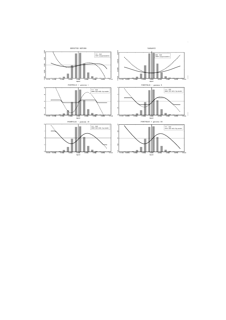
Figure 1: Expected return, expected squared return and portfolio choice - Rule 1

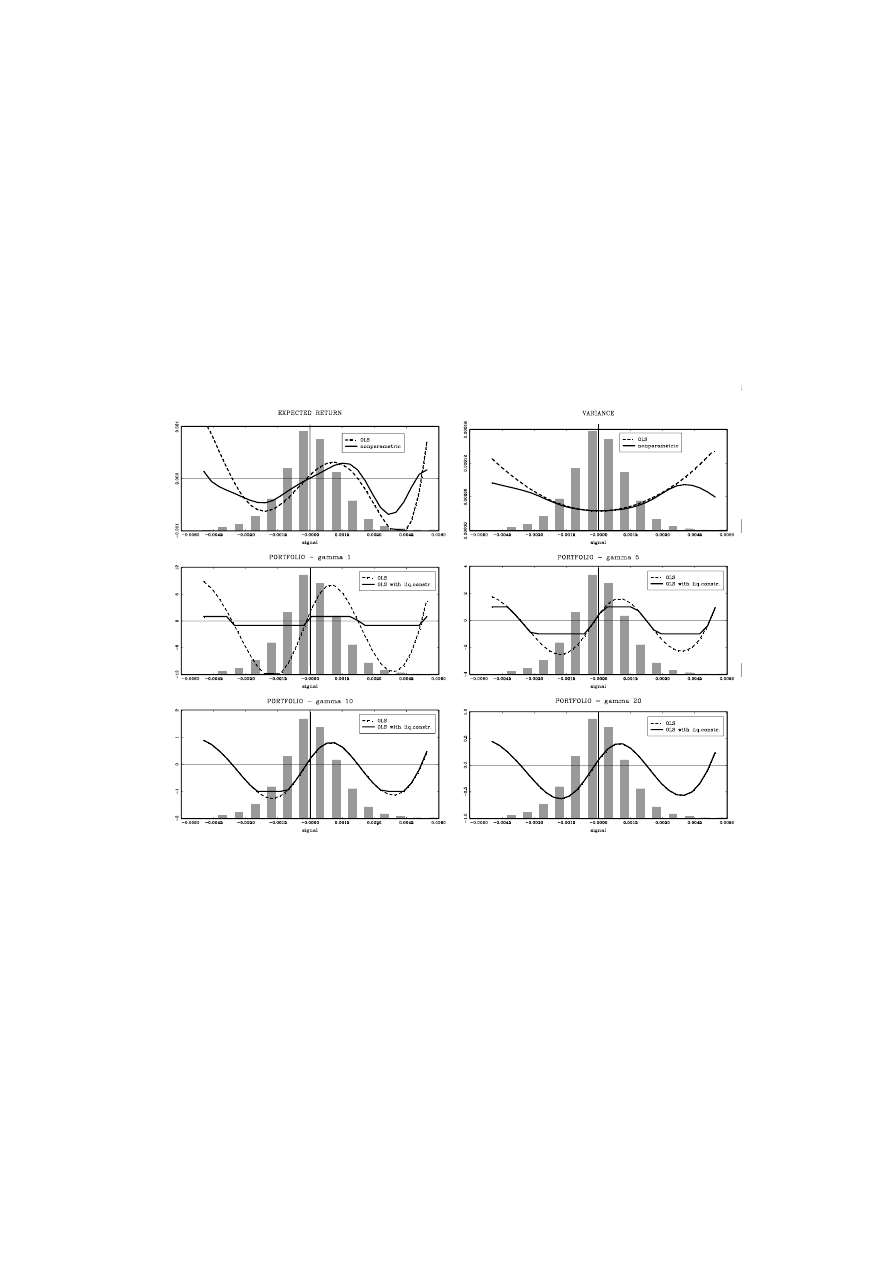
Figure 2: Expected return, expected squared return and portfolio choice - Rule 2

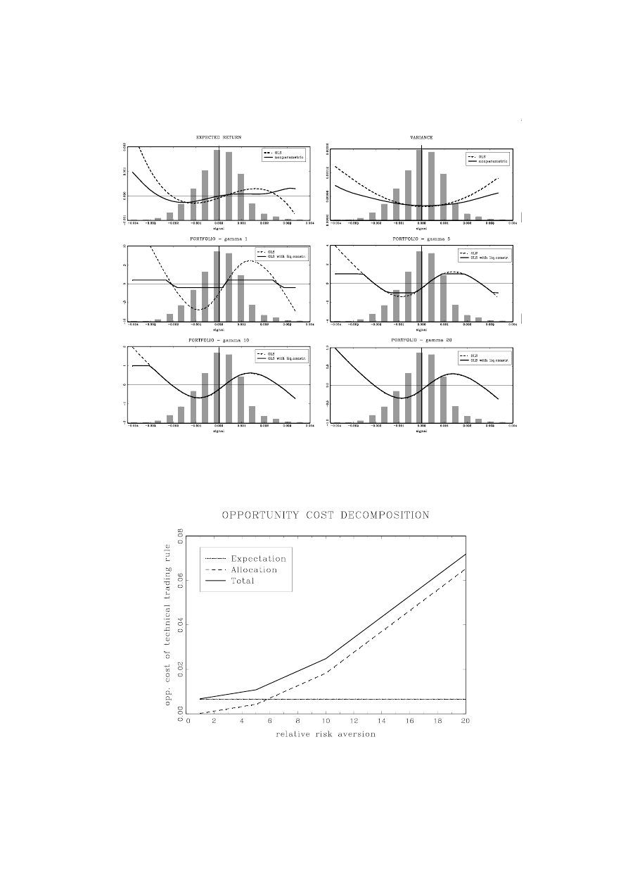
Figure 3: Expected return, expected squared return and portfolio choice - Rule 3

Figure 4: Opportunity cost decomposition. DEM/USA, Rule 1

Table 2: In-sample analysis of certainty equivalent and cost decomosition of tech-
nical trading rules. Rule 1: S=10, L=50

CRRA=1

CRRA=5

CRRA=10

CRRA=20

DEM/USD: p

= 3, p

= 2

ceq

0.04872

0.03063

0.01693

0.00855

ceq

0.04855

0.02638

0.00133

0.05675

ceq

0.04199

0.04872

0.00788

0.06330

EXP

0.00656

ALL

0.00018

0.00425

0.01826

0.06529

0.00673

0.01081

0.02481

0.07185

GBP/USD: p

= 4, p

= 6

ceq

0.03565

0.02075

0.01120

0.00607

ceq

0.03551

0.01727

-0.00554

-0.05115

ceq

0.02687

0.00863

-0.01418

-0.05979

EXP

0.00864

ALL

0.00014

0.00348

0.01674

0.05722

0.00878

0.01212

0.02538

0.06586

JPY/USD: p

= 3, p

= 4

ceq

0.05550

0.03739

0.02413

0.01254

ceq

0.05533

0.03274

0.00450

-0.05196

ceq

0.04312

0.02053

-0.00771

-0.06417

EXP

0.01221

ALL

0.00018

0.00466

0.01963

0.06450

0.01239

0.01687

0.03184

0.07671

CHF/USD: p

= 3, p

= 2

ceq

0.05006

0.02846

0.01550

0.00798

ceq

0.04978

0.02120

-0.01452

-0.08596

ceq

0.03354

0.00496

-0.03076

-0.10221

EXP

0.01624

ALL

0.00028

0.00725

0.03002

0.09394

0.01652

0.02350

0.04627

0.11018

The parameters p

and p

denote the maximal order of the Taylor expansions

used in the estimation.
ceq

denotes the certainty equivalent of strategy i for a trader with constant rel-

ative risk aversion denoted in the top of the table. ceq

denotes the certainty

equivalent based on the optimal trading strategy. ceq

denotes the certainty

equivalent when the risk averse trader uses the risk neutral optimal portfolio,
and ceq

denotes the certainty equivalent for a risk averse trader following

the technical trading rule.
All entries are in per annum terms.

Table 3: In-sample analysis of certainty equivalent and cost decomosition of tech-
nical trading rules. Rule 2: S=20, L=100

CRRA=1

CRRA=5

CRRA=10

CRRA=20

DEM/USD: p

= 5, p

= 2

ceq

0.06572

0.04660

0.02928

0.01484

ceq

0.06560

0.04338

0.01560

-0.03994

ceq

0.05161

0.02939

0.00161

-0.05393

EXP

0.01399

ALL

0.00012

0.00322

0.01367

0.05478

0.01411

0.01721

0.02766

0.06877

GBP/USD: p

= 2, p

= 4

ceq

0.02646

0.01256

0.00641

0.00321

ceq

0.02631

0.00798

-0.01493

-0.06076

ceq

0.01291

-0.00542

-0.02833

-0.07416

EXP

0.01340

ALL

0.00015

0.00458

0.02135

0.06396

0.01355

0.01798

0.03474

0.07736

JPY/USD: p

= 3, p

= 2

ceq

0.06492

0.04589

0.03015

0.01585

ceq

0.06477

0.04210

0.01376

-0.04291

ceq

0.05371

0.03104

0.00271

-0.05396

EXP

0.01106

ALL

0.00015

0.00379

0.01639

0.05875

0.01121

0.01485

0.02745

0.06981

CHF/USD: p

= 1, p

= 4

ceq

0.02565

0.00933

0.00467

0.00234

ceq

0.02515

-0.00354

-0.03941

-0.11114

ceq

0.01451

-0.01418

-0.05005

-0.12178

EXP

0.01064

ALL

0.00050

0.01287

0.04408

0.11348

0.01114

0.02351

0.05472

0.12412

The parameters p

and p

denote the maximal order of the Taylor expansions

used in the estimation.
ceq

denotes the certainty equivalent of strategy i for a trader with constant rel-

ative risk aversion denoted in the top of the table. ceq

denotes the certainty

equivalent based on the optimal trading strategy. ceq

denotes the certainty

equivalent when the risk averse trader uses the risk neutral optimal portfolio,
and ceq

denotes the certainty equivalent for a risk averse trader following

the technical trading rule.
All entries are in per annum terms.

Table 4: In-sample analysis of certainty equivalent and cost decomosition of tech-
nical trading rules. Rule 3: S=40, L=200

CRRA=1

CRRA=5

CRRA=10

CRRA=20

DEM/USD: p

= 3, p

= 2

ceq

0.04158

0.02422

0.01289

0.00656

ceq

0.04139

0.01938

0.00812

0.06313

ceq

0.03208

0.01008

0.01743

0.07244

EXP

0.00931

ALL

0.00020

0.00483

0.02101

0.06969

0.00951

0.01414

0.03032

0.07900

GBP/USD: p

= 5, p

= 4

ceq

0.04363

0.02821

0.01805

0.01032

ceq

0.04357

0.02513

0.00208

-0.04401

ceq

0.02388

0.00544

-0.01743

-0.06370

EXP

0.01969

ALL

0.00007

0.00308

0.01596

0.05433

0.01975

0.02277

0.03565

0.07402

JPY/USD: p

= 3, p

= 2

ceq

0.04271

0.02679

0.01627

0.00818

ceq

0.04245

0.01960

-0.00897

-0.06610

ceq

0.03641

0.01356

-0.01501

-0.07214

EXP

0.00604

ALL

0.00026

0.00713

0.02523

0.07428

0.00630

0.01324

0.03128

0.08033

CHF/USD: p

= 3, p

= 5

ceq

0.04924

0.02752

0.01498

0.00780

ceq

0.04900

0.02053

-0.01505

-0.08620

ceq

0.03489

0.00643

-0.02915

-0.10031

EXP

0.01411

ALL

0.00024

0.00699

0.03002

0.09401

0.01435

0.02109

0.04413

0.10811

The parameters p

and p

denote the maximal order of the Taylor expansions

used in the estimation.
ceq

denotes the certainty equivalent of strategy i for a trader with constant rel-

ative risk aversion denoted in the top of the table. ceq

denotes the certainty

equivalent based on the optimal trading strategy. ceq

denotes the certainty

equivalent when the risk averse trader uses the risk neutral optimal portfolio,
and ceq

denotes the certainty equivalent for a risk averse trader following

the technical trading rule.
All entries are in per annum terms.

Table 5: Dynamic estimation of certainty equivalent and cost decomosition of
technical trading rules. Rule 1: S=10, L=50

CRRA=1

CRRA=5

CRRA=10

CRRA=20

DEM/USD: p

= 3, p

= 2

ceq

0.08300

0.06459

0.04627

0.02673

ceq

0.08290

0.06216

0.03625

0.01559

ceq

0.06544

0.04471

0.01879

0.03304

EXP

0.01746

ALL

0.00010

0.00242

0.01003

0.04232

0.01756

0.01988

0.02748

0.05977

GBP/USD: p

= 4, p

= 6

ceq

0.06443

0.04915

0.03556

0.02239

ceq

0.06435

0.04688

0.02504

-0.01863

ceq

0.03843

0.02096

-0.00087

-0.04455

EXP

0.02592

ALL

0.00009

0.00227

0.01052

0.04102

0.02600

0.02818

0.03643

0.06694

JPY/USD: p

= 3, p

= 4

ceq

0.07545

0.05784

0.04172

0.02356

ceq

0.07534

0.05511

0.02982

-0.02076

ceq

0.06344

0.04321

0.01792

-0.03266

EXP

0.01190

ALL

0.00011

0.00273

0.01190

0.04432

0.01201

0.01463

0.02381

0.05622

CHF/USD: p

= 3, p

= 2

ceq

0.09748

0.07226

0.05002

0.02972

ceq

0.09732

0.06809

0.03156

-0.04151

ceq

0.05656

0.02733

-0.00921

-0.08227

EXP

0.04076

ALL

0.00016

0.00417

0.01847

0.07123

0.04092

0.04493

0.05923

0.11199

The parameters p

and p

denote the maximal order of the Taylor expansions

used in the estimation.
ceq

denotes the certainty equivalent of strategy i for a trader with constant rel-

ative risk aversion denoted in the top of the table. ceq

denotes the certainty

equivalent based on the optimal trading strategy. ceq

denotes the certainty

equivalent when the risk averse trader uses the risk neutral optimal portfolio,
and ceq

denotes the certainty equivalent for a risk averse trader following

the technical trading rule.
All entries are in per annum terms.

Table 6: Dynamic estimation of certainty equivalent and cost decomosition of
technical trading rules. Rule 2: S=20, L=100

CRRA=1

CRRA=5

CRRA=10

CRRA=20

DEM/USD: p

= 5, p

= 2

ceq

0.09484

0.07647

0.05796

0.03584

ceq

0.09475

0.07426

0.04865

-0.00258

ceq

0.08419

0.06370

0.03809

-0.01314

EXP

0.01056

ALL

0.00008

0.00221

0.00931

0.03842

0.01064

0.01276

0.01987

0.04898

GBP/USD: p

= 2, p

= 4

ceq

0.05701

0.04218

0.03013

0.01864

ceq

0.05692

0.03965

0.01806

-0.02512

ceq

0.02548

0.00820

-0.01339

-0.05657

EXP

0.03144

ALL

0.00009

0.00253

0.01207

0.04376

0.03153

0.03397

0.04352

0.07520

JPY/USD: p

= 3, p

= 2

ceq

0.07296

0.05601

0.04130

0.02475

ceq

0.07284

0.05279

0.02772

-0.02243

ceq

0.05461

0.03456

0.00948

-0.04066

EXP

0.01823

ALL

0.00012

0.00323

0.01358

0.04718

0.01835

0.02146

0.03181

0.06541

CHF/USD: p

= 1, p

= 4

ceq

0.04483

0.02356

0.01290

0.00651

ceq

0.04448

0.01500

-0.02185

-0.09555

ceq

0.02164

-0.00785

-0.04470

-0.11840

EXP

0.02284

ALL

0.00035

0.00856

0.03475

0.10206

0.02319

0.03141

0.05759

0.12490

The parameters p

and p

denote the maximal order of the Taylor expansions

used in the estimation.
ceq

denotes the certainty equivalent of strategy i for a trader with constant rel-

ative risk aversion denoted in the top of the table. ceq

denotes the certainty

equivalent based on the optimal trading strategy. ceq

denotes the certainty

equivalent when the risk averse trader uses the risk neutral optimal portfolio,
and ceq

denotes the certainty equivalent for a risk averse trader following

the technical trading rule.
All entries are in per annum terms.

Table 7: Dynamic estmation of certainty equivalent and cost decomosition of tech-
nical trading rules. Rule 3: S=40, L=200

CRRA=1

CRRA=5

CRRA=10

CRRA=20

DEM/USD: p

= 3, p

= 2

ceq

0.05654

0.03985

0.02612

0.01486

ceq

0.05642

0.03660

0.01183

0.03770

ceq

0.04682

0.02701

0.00224

0.04730

EXP

0.00960

ALL

0.00012

0.00325

0.01428

0.05256

0.00972

0.01285

0.02388

0.06216

GBP/USD: p

= 5, p

= 4

ceq

0.08010

0.06466

0.04995

0.03381

ceq

0.08004

0.06309

0.04190

-0.00048

ceq

0.04229

0.02534

0.00415

-0.03823

EXP

0.03775

ALL

0.00006

0.00157

0.00805

0.03428

0.03781

0.03932

0.04580

0.07203

JPY/USD: p

= 3, p

= 2

ceq

0.05941

0.04480

0.03315

0.02030

ceq

0.05919

0.03908

0.01394

-0.03634

ceq

0.03672

0.01661

-0.00853

-0.05880

EXP

0.02247

ALL

0.00021

0.00572

0.01920

0.05663

0.02269

0.02819

0.04167

0.07910

CHF/USD: p

= 3, p

= 5

ceq

0.07474

0.05126

0.03286

0.01865

ceq

0.07454

0.04589

0.01007

-0.06155

ceq

0.05611

0.00275

-0.00836

-0.07998

EXP

0.01843

ALL

0.00021

0.00538

0.02279

0.08020

0.01864

0.02381

0.04122

0.09863

The parameters p

and p

denote the maximal order of the Taylor expansions

used in the estimation.
ceq

denotes the certainty equivalent of strategy i for a trader with constant rel-

ative risk aversion denoted in the top of the table. ceq

denotes the certainty

equivalent based on the optimal trading strategy. ceq

denotes the certainty

equivalent when the risk averse trader uses the risk neutral optimal portfolio,
and ceq

denotes the certainty equivalent for a risk averse trader following

the technical trading rule.
All entries are in per annum terms.

Table 8: Out-of-sample certainty equivalent and cost decomposition of technical
trading rules. Rule 1: S=10, L=50

CRRA=1

CRRA=5

CRRA=10

CRRA=20

DEM/USD: p

= 3, p

= 2

ceq

0.06515

0.04079

0.02045

0.01149

ceq

0.06376

0.04090

0.01233

-0.04482

ceq

0.04125

0.01837

-0.01023

-0.06743

EXP

0.02250

ALL

0.00140

0.00008

0.00819

0.05642

0.02390

0.02242

0.03068

0.07892

GBP/USD: p

= 4, p

= 6

ceq

0.03140

0.02170

0.01410

0.01082

ceq

0.02802

0.00856

-0.01577

-0.06442

ceq

0.02786

0.00835

-0.01605

-0.06485

EXP

0.00014

ALL

0.00339

0.01321

0.03001

0.07552

0.00354

0.01336

0.03016

0.07567

JPY/USD: p

= 3, p

= 4

ceq

0.07707

0.05626

0.03973

0.02183

ceq

0.07669

0.05217

0.02153

-0.03976

ceq

0.05449

0.03000

-0.00618

-0.06185

EXP

0.02221

ALL

0.00375

0.00406

0.01814

0.06148

0.02258

0.02627

0.04034

0.08368

CHF/USD: p

= 3, p

= 4

ceq

0.07492

0.04566

0.02447

0.01538

ceq

0.06883

0.03938

0.00256

-0.07107

ceq

0.05300

0.00236

-0.01322

-0.08679

EXP

0.01584

ALL

0.00609

0.00625

0.02185

0.08633

0.02193

0.02209

0.03769

0.10217

The parameters p

and p

denote the maximal order of the Taylor expansions

used in the estimation.
ceq

denotes the certainty equivalent of strategy i for a trader with constant rel-

ative risk aversion denoted in the top of the table. ceq

denotes the certainty

equivalent based on the optimal trading strategy. ceq

denotes the certainty

equivalent when the risk averse trader uses the risk neutral optimal portfolio,
and ceq

denotes the certainty equivalent for a risk averse trader following

the technical trading rule.
All entries are in per annum terms.

Table 9: Out-of-sample certainty equivalent and cost decomposition of technical
trading rules. Rule 2: S=20, L=100

CRRA=1

CRRA=5

CRRA=10

CRRA=20

DEM/USD: p

= 5, p

= 2

ceq

0.06192

0.04303

0.02490

0.01362

ceq

0.06118

0.03826

0.00962

-0.04766

ceq

0.03582

0.01288

-0.01579

-0.07313

EXP

0.02536

ALL

0.00075

0.00479

0.01533

0.06140

0.02611

0.03015

0.04069

0.08675

GBP/USD: p

= 2, p

= 4

ceq

0.01417

0.00482

0.00072

-0.00182

ceq

0.01267

-0.00689

-0.03133

-0.08021

ceq

0.03418

0.01467

-0.00971

-0.05847

EXP

-0.02146

-0.02150

ALL

0.00149

0.01165

0.03192

0.07815

-0.02001

-0.00985

0.01043

0.05665

JPY/USD: p

= 3, p

= 2

ceq

0.06967

0.06002

0.03879

0.02000

ceq

0.06601

0.04151

0.01087

-0.05039

ceq

0.05228

0.02779

-0.00283

-0.06406

EXP

0.01373

ALL

0.00365

0.01850

0.02788

0.07032

0.01739

0.03223

0.04162

0.08406

CHF/USD: p

= 1, p

= 4

ceq

0.02086

0.01335

0.00987

0.00540

ceq

0.01726

-0.01194

-0.04843

-0.12141

ceq

0.03209

0.00290

-0.03359

-0.10656

EXP

-0.01483

ALL

0.00361

0.02528

0.05829

0.12679

-0.01122

0.01046

0.04346

0.11196

The parameters p

and p

denote the maximal order of the Taylor expansions

used in the estimation.
ceq

denotes the certainty equivalent of strategy i for a trader with constant rel-

ative risk aversion denoted in the top of the table. ceq

denotes the certainty

equivalent based on the optimal trading strategy. ceq

denotes the certainty

equivalent when the risk averse trader uses the risk neutral optimal portfolio,
and ceq

denotes the certainty equivalent for a risk averse trader following

the technical trading rule.
All entries are in per annum terms.

Table 10: Out of sample certainty equivalent and cost decomposition of technical
trading rules. Rule 3: S=40, L=200

CRRA=1

CRRA=5

CRRA=10

CRRA=20

DEM/USD: p

= 3, p

= 2

ceq

0.05256

0.02888

0.01988

0.00950

ceq

0.05194

0.02910

0.00054

0.05657

ceq

0.01637

-0.00649

-0.03506

0.09221

EXP

0.03557

ALL

0.00062

-0.00020

0.01937

0.06614

0.03619

0.03537

0.05494

0.10171

GBP/USD: p

= 5, p

= 4

ceq

0.03671

0.01919

0.01125

0.00848

ceq

0.03565

0.01605

-0.00845

-0.05745

ceq

0.03055

0.01085

-0.01378

-0.06304

EXP

0.00507

ALL

0.00108

0.00327

0.01996

0.06645

0.00616

0.00834

0.02503

0.07152

JPY/USD: p

= 3, p

= 2

ceq

0.03977

0.02901

0.01916

0.01249

ceq

0.03788

0.01334

-0.01734

-0.07870

ceq

0.02292

-0.00152

-0.03207

-0.09318

EXP

0.01498

ALL

0.00187

0.01555

0.03625

0.09069

0.01685

0.03053

0.05123

0.10567

CHF/USD: p

= 3, p

= 5

ceq

0.04816

0.03527

0.02827

0.01596

ceq

0.04003

0.01074

-0.02588

-0.09910

ceq

0.03261

0.00335

-0.03322

-0.10637

EXP

0.00742

ALL

0.00812

0.02449

0.05407

0.11490

0.01555

0.03192

0.06149

0.12232

The parameters p

and p

denote the maximal order of the Taylor expansions

used in the estimation.
ceq

denotes the certainty equivalent of strategy i for a trader with constant rel-

ative risk aversion denoted in the top of the table. ceq

denotes the certainty

equivalent based on the optimal trading strategy. ceq

denotes the certainty

equivalent when the risk averse trader uses the risk neutral optimal portfolio,
and ceq

denotes the certainty equivalent for a risk averse trader following

the technical trading rule.
All entries are in per annum terms.

Publications in the Report Series Research

∗

in Management

ERIM Research Program: “Finance and Accounting”

2003

COMMENT, Risk Aversion and Skewness Preference

Thierry Post and Pim van Vliet
ERS-2003-009-F&A

http://hdl.handle.net/1765/319

International Portfolio Choice: A Spanning Approach
Ben Tims, Ronald Mahieu

ERS-2003-011-F&A

http://hdl.handle.net/1765/276

Portfolio Return Characteristics Of Different Industries
Igor Pouchkarev, Jaap Spronk, Pim van Vliet

ERS-2003-014-F&A

http://hdl.handle.net/1765/272

Asset prices and omitted moments

A stochastic dominance analysis of market efficiency

Thierry Post

ERS-2003-017-F&A

http://hdl.handle.net/1765/430

A Multidimensional Framework for Financial-Economic Decisions

Winfried Hallerbach & Jaap Spronk
ERS-2003-021-F&A

http://hdl.handle.net/1765/321

A Range-Based Multivariate Model for Exchange Rate Volatility
Ben Tims, Ronald Mahieu

ERS-2003-022-F&A

http://hdl.handle.net/1765/282

Macro factors and the Term Structure of Interest Rates

Hans Dewachter and Marco Lyrio

ERS-2003-037-F&A

http://hdl.handle.net/1765/324

The effects of decision flexibility in the hierarchical investment decision process

Winfried Hallerbach, Haikun Ning, Jaap Spronk

ERS-2003-047-F&A

http://hdl.handle.net/1765/426

∗

A complete overview of the ERIM Report Series Research in Management:

http://www.erim.eur.nl

ERIM

Research

Programs:

LIS Business Processes, Logistics and Information Systems

ORG Organizing for Performance

MKT

Marketing

F&A Finance and Accounting

STR Strategy and Entrepreneurship

Takeover defenses and IPO firm value in the Netherlands

Peter Roosenboom, Tjalling van der Goot

ERS-2003-049-F&A

http://hdl.handle.net/1765/433

The Cost of Technical Trading Rules in the Forex Market: A Utility-based Evaluation

Hans Dewachter and Marco Lyrio
ERS-2003-052-F&A

Wyszukiwarka

Podobne podstrony:
John Murphy s Ten Laws of Technical Trading
Why Most People Lose Money in the Forex Market (Booker)
Forex For Everyone Learn To Trade The Forex Market Like A Professional
The Code of Honor or Rules for the Government of Principals and Seconds in Duelling by John Lyde Wil
There are a lot of popular culture references in the show
Capability of high pressure cooling in the turning of surface hardened piston rods
Zen & the Art of Mayhem Optional Rules
DV8 Physical Theatre the cost of living, STUDIA Pedagogika resocjalizacyjna
The algorithm of solving differential equations in continuous model of tall buildings subjected to c
Domains of Adventure The Museum of Infamous Heroism Rules Appendix
RES , Out of hospital airway management in the United States
Identifying Active Trading Strategies in the Bitcoin Market
The energy consumption and economic costs of different vehicles used in transporting woodchips Włoch
The Pernicious Blend of Rumination and Fearlessness in NSSI
The Presentation of Self and Other in Nazi Propaganda
In the context of globalization, Calligraphy’s function in poetic dwelling
Role of the Structure of Heterogeneous Condensed Mixtures in the Formation of Agglomerates
Suke Wolton Lord Hailey, the Colonial Office and the Politics of Race and Empire in the Second Worl

więcej podobnych podstron