Using Simulink
®
and Stateflow
TM
in Automotive Applications
S
IMULINK
-S
TATEFLOW
T
ECHNICAL
E
XAMPLES
This book includes nine examples that represent typical design tasks of an automotive engineer. It
shows how The MathWorks modeling and simulation tools, Simulink
®
and Stateflow,
TM
facilitate
the design of automotive control systems. Each example explains the principles of the physical sit-
uation, and presents the equations that represent the system. The examples show how to proceed
from the physical equations to the Simulink block diagram. Once the Simulink model has been
completed, we run the simulation, analyze the results, and draw conclusions from the study.
Abstract


U
SING
S
IMULINK AND
S
TATEFLOW IN
A
UTOMOTIVE
A
PPLICATIONS
3
T
ABLE OF
C
ONTENTS
Introduction ....................................................................................................................... 4
System Models in Simulink................................................................................................ 7
I. Engine Model.............................................................................................................. 8
II. Anti-Lock Braking System........................................................................................ 18
III. Clutch Engagement Model....................................................................................... 23
IV. Suspension System.................................................................................................... 31
V. Hydraulic Systems .................................................................................................... 35
System Models in Simulink with Stateflow Enhancements .......................................... 49
VI. Fault-Tolerant Fuel Control System ........................................................................ 50
VII. Automatic Transmission Control............................................................................. 61
VIII. Electrohydraulic Servo Control ............................................................................... 71
IX. Modeling Stick-Slip Friction .................................................................................... 84

4
S
IMULINK
-S
TATEFLOW
T
ECHNICAL
E
XAMPLES
I
NTRODUCTION
Summary
Automotive engineers have found simulation to be a vital tool in the timely and cost-effective
development of advanced control systems. As a design tool, Simulink has become the standard for
excellence through its flexible and accurate modeling and simulation capabilities. As a result of its open
architecture, Simulink allows engineers to create custom block libraries so they can leverage each other’s
work. By sharing a common set of tools and libraries, engineers can work together effectively within
individual work groups and throughout the entire engineering department.
In addition to the efficiencies achieved by Simulink, the design process can also benefit from Stateflow, an
interactive design tool that enables the modeling and simulation of complex reactive systems. Tightly
integrated with Simulink, Stateflow allows engineers to design embedded control systems by giving them
an efficient graphical technique to incorporate complex control and supervisory logic within their
Simulink models.
This booklet describes nine automotive design examples that illustrate the strengths of Simulink and
Stateflow in accelerating and facilitating the design process.
Examples
The examples cited in this booklet consist of application design tasks typically encountered in
Description
the automotive industry. We present a variety of detailed models including the underlying
equations, block diagrams, and simulation results. The material may serve as a starting point for the
new Simulink user or as a reference for the more experienced user. In the models, we propose approaches
for model development, present solutions to challenging problems, and illustrate some of the most
common design uses of Simulink and Stateflow today.
The applications and models described in this booklet include the following examples using Simulink
alone:
I.
Engine Model
engine.mdl
— open-loop simulation
enginewc.mdl
— closed-loop simulation
II.
Anti-Lock Braking System
absbrake.mdl
III.
Clutch Engagement Model
clutch.mdl
IV.
Suspension System
suspn.mdl
V.
Hydraulic Systems
hydcyl
.
mdl
— Pump and actuator assembly
hydcyl4
.
mdl
— Four-cylinder model
hydrod
.
mdl
— Two-cylinder model with load constraints

U
SING
S
IMULINK AND
S
TATEFLOW IN
A
UTOMOTIVE
A
PPLICATIONS
5
The following applications and models use Simulink enhanced with Stateflow:
VI.
Fault-Tolerant Fuel Control System
fuelsys
.
mdl
VII.
Automatic Transmission Control
sf
_
car
.
mdl
VIII.
Electrohydraulic Servo Control
sf
_
electrohydraulic
.
mdl
IX.
Modeling Stick-Slip Friction
sf
_
stickslip
.
mdl
Simulink
The models used in this book are available via ftp at
Model Files
ftp://ftp.mathworks.com/pub/product-info/examples/autobook.zip
. This zip file contains the set
of MDL, MAT, and M-files containing Simulink models that users can explore and build upon. The
included files require M
ATLAB®
5.1, Simulink 2.1, and Stateflow 1.0. Models for these applications can be
opened in Simulink by typing the name of the model at the M
ATLAB
command prompt. M
ATLAB
,
Simulink, and Stateflow are not included with this booklet. To obtain a copy of M
ATLAB
, Simulink, and
Stateflow, or for a diskette containing the model files, please contact your representative at The
MathWorks.
Acknowledgments
The engine model is based on published findings by Crossley and Cook (1991)(1). We’d like to thank
Ken Butts and Jeff Cook of the Ford Motor Company for permission to include this model and for
subsequent help in building the model in Simulink.
The clutch and hydraulic cylinder models are based on equations provided by General Motors. We’d like
to thank Eric Gassenfeit of General Motors for permission to include these models.
The vehicle suspension model was written by David MacClay of Cambridge Control Ltd.
The simple three-state engine model and the set of icons that are relevant for automotive modeling were
provided by Modular Systems. A far more detailed engine model may be purchased directly from Modular
Systems.
Contact
The MathWorks technical personnel specializing in automotive solutions can be reached via e-mail
Information
at the following addresses:
Stan Quinn
squinn@mathworks.com
Andy Grace
agrace@mathworks.com
Paul Barnard
pbarnard@mathworks.com
Larry Michaels
lmichaels@mathworks.com
Bill Aldrich
baldrich@mathworks.com

6
S
IMULINK
-S
TATEFLOW
T
ECHNICAL
E
XAMPLES
Or contact any of our international distributors and resellers directly. See the back page for additional
contact information.
Both Modular Systems and Cambridge Control Ltd. offer consulting services in automotive modeling.
They can be reached as follows:
Attention: Robert W. Weeks
Modular Systems
714 Sheridan Road
Evanston, IL 60202-2502 USA
Tel: 708-869-2023
E-mail: bobweeks@ix.netcom.com
Attention: Sham Ahmed
Cambridge Control Ltd.
Newton House
Cambridge Business Park
Cowley Road
Cambridge, DB4 4WZ UK
011/44-1223-423-2
E-mail: Sham@camcontrol.co.uk

U
SING
S
IMULINK AND
S
TATEFLOW IN
A
UTOMOTIVE
A
PPLICATIONS
7
System Models in Simulink

8
S
IMULINK
-S
TATEFLOW
T
ECHNICAL
E
XAMPLES
I. E
NGINE
M
ODEL
Summary
This example presents a model of a four-cylinder spark ignition engine and demonstrates Simulink’s
capabilities to model an internal combustion engine from the throttle to the crankshaft output. We used
well-defined physical principles supplemented, where appropriate, with empirical relationships that
describe the system’s dynamic behavior without introducing unnecessary complexity.
Overview
This example describes the concepts and details surrounding the creation of engine models with emphasis
on important Simulink modeling techniques. The basic model uses the enhanced capabilities of
Simulink 2 to capture time-based events with high fidelity. Within this simulation, a triggered
subsystem models the transfer of the air-fuel mixture from the intake manifold to the cylinders via
discrete valve events. This takes place concurrently with the continuous-time processes of intake flow,
torque generation and acceleration. A second model adds an additional triggered subsystem that provides
closed-loop engine speed control via a throttle actuator.
These models can be used as standalone engine simulations. Or, they can be used within a larger system
model, such as an integrated vehicle and powertrain simulation, in the development of a traction control
system.
Model Description
This model, based on published results by Crossley and Cook (1991), describes the simulation of a four-
cylinder spark ignition internal combustion engine. The Crossley and Cook work also shows how a
simulation based on this model was validated against dynamometer test data.
The ensuing sections (listed below) analyze the key elements of the engine model that were identified by
Crossley and Cook:
•
Throttle
•
Intake manifold
•
Mass flow rate
•
Compression stroke
•
Torque generation and acceleration
Note: Additional components can be added to the model to provide greater accuracy in simulation and to
more closely replicate the behavior of the system.
Analysis
T
HROTTLE
and Physics
The first element of the simulation is the throttle body. Here, the control input is the angle of the throttle
plate. The rate at which the model introduces air into the intake manifold can be expressed as the product
of two functions—one, an empirical function of the throttle plate angle only; and the other, a function of
the atmospheric and manifold pressures. In cases of lower manifold pressure (greater vacuum), the flow
rate through the throttle body is sonic and is only a function of the throttle angle. This model accounts for

U
SING
S
IMULINK AND
S
TATEFLOW IN
A
UTOMOTIVE
A
PPLICATIONS
9
this low pressure behavior with a switching condition in the compressibility equations shown in
Equation 1.1.
˙
( ) (
)
( )
.
.
.
.
(
)
,
,
,
,
m
f
g P
f
g P
P
P
P
P P
P
P
P
P
P
P P
P
P
P
P
P
ai
m
m
m
amb
amb
m amb
m
amb
m
amb
m
m amb
amb
amb
m
amb
=
=
=
−
+
−
=
=
≤
−
≤
≤
−
−
≤
≤
−
θ
θ
θ
θ
θ
θ
mass flow rate into manifold (g/s) where,
throttle angle (deg)
2 821
0 05231
0 10299
0 00063
1
2
2
2
2
2
1
2
3
2
2
m
m
amb
m
amb
P
P
P
≥
=
=
2
manifold pressure (bar)
ambient (atmospheric)
pressure (bar)
Equation
1.1
Intake Manifold
The simulation models the intake manifold as a differential equation for the manifold pressure. The
difference in the incoming and outgoing mass flow rates represents the net rate of change of air mass with
respect to time. This quantity, according to the ideal gas law, is proportional to the time derivative of the
manifold pressure. Note that, unlike the model of Crossley and Cook, 1991(1) (see also references 3
through 5), this model doesn’t incorporate exhaust gas recirculation (EGR), although this can easily be
added.
˙
˙
˙
P
RT
V
m
m
m
m
ai
ao
=
−
(
)
Equation 1.2
where,
R
T
V
m
P
m
ao
m
=
=
=
=
=
specific gas constant
temerature ( K)
manifold volume (m )
mass flow rate of air out of the manifold (g/s)
rate of change of manifold pressure (bar/s)
3
˚
˙
˙
Intake Mass Flow Rate
The mass flow rate of air that the model pumps into the cylinders from the manifold is described in
Equation 1.3 by an empirically derived equation. This mass rate is a function of the manifold pressure
and the engine speed.
˙
.
.
.
.
m
NP
NP
N P
ao
m
m
m
= −
+
−
+
0 366
0 08979
0 0337
0 0001
2
2
Equation 1.3

10
S
IMULINK
-S
TATEFLOW
T
ECHNICAL
E
XAMPLES
where,
N
P
m
=
=
engine speed (rad/s)
manifold pressure (bar)
To determine the total air charge pumped into the cylinders, the simulation integrates the mass flow rate
from the intake manifold and samples it at the end of each intake stroke event. This determines the total
air mass that is present in each cylinder after the intake stroke and before compression.
Compression Stroke
In an inline four-cylinder four-stroke engine, 180
°
of crankshaft revolution separate the ignition of each
successive cylinder. This results in each cylinder firing on every other crank revolution. In this model,
the intake, compression, combustion, and exhaust strokes occur simultaneously (at any given time, one
cylinder is in each phase). To account for compression, the combustion of each intake charge is delayed
by 180
°
of crank rotation from the end of the intake stroke.
Torque Generation and Acceleration
The final element of the simulation describes the torque developed by the engine. An empirical
relationship dependent upon the mass of the air charge, the air/fuel mixture ratio, the spark advance, and
the engine speed is used for the torque computation.
Torque
m
A F
A F
N
N
N
m
m
eng
a
a
a
= −
+
+
−
+
−
+
−
+
+
−
181 3 379 36
21 91
0 85
0 26
0 0028
0 027
0 000107
0 00048
2 55
0 05
2
2
2
2
.
.
. ( / )
.
( / )
.
.
.
.
.
.
.
σ
σ
σ
σ
σ
Equation 1.4
where,
m
A F
Torque
a
eng
=
=
=
=
mass of air in cylinder for combustion (g)
air to fuel ratio
spark advance (degrees before top - dead - center
torque produced by the engine (Nm)
/
σ
The engine torque less the net load torque results in acceleration.
JN
Torque
Torque
eng
load
˙
=
−
Equation 1.5
where,
J
= Engine rotational moment of inertia (kg-m
2
)
˙
N
= Engine acceleration (rad/s
2
)
U
SING
S
IMULINK AND
S
TATEFLOW IN
A
UTOMOTIVE
A
PPLICATIONS
11
Modeling —
We incorporated the model elements described above into an engine model using Simulink. The
The Open-Loop
following sections describe the decisions we made for this implementation and the key Simulink elements
Simulation
used. This section shows how to implement a complex nonlinear engine model easily and quickly in the
Simulink environment. We developed this model in conjunction with Ken Butts, Ford Motor Company (2).
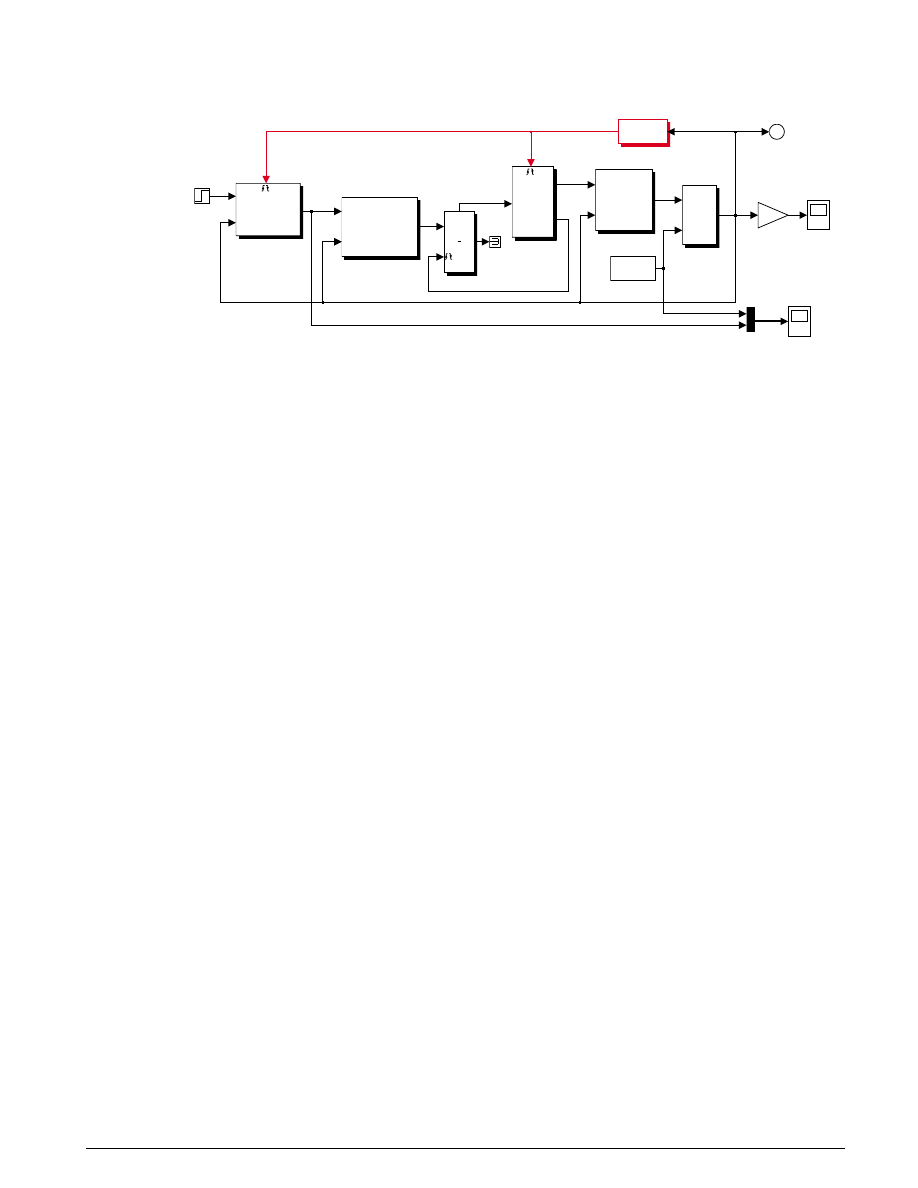
Figure 1.1 shows the top level of the Simulink model. Note that, in general, the major blocks correspond
to the high-level list of functions given in the model description in the preceding summary. Taking
advantage of Simulink’s hierarchical modeling capabilities, most of the blocks in Figure 1.1 are made up
of smaller blocks. The following paragraphs describe these smaller blocks.
choose Start from
the Simulation
menu to run
Engine Timing Model in Simulink 2
A Demonstration of Triggered Subsystems
1
crank speed
(rad/sec)
N
edge180
valve timing
throttle deg (purple)
load torque Nm (yellow)
throttle
(degrees)
30/pi
rad/s
to
rpm
Teng
Tload
N
Vehicle
Dynamics
Throttle Ang.
Engine Speed, N
Mass Airflow Rate
Throttle & Manifold
Mux
s
1
Intake
Engine
Speed
(rpm)
Load
Drag Torque
mass(k+1)
mass(k)
trigger
Compression
Air Charge
N
Torque
Combustion
Figure 1.1: The top level of the Simulink engine model
Throttle/Manifold
Simulink models for the throttle and intake manifold subsystems are shown in Figure 1.2. The throttle
valve behaves in a nonlinear manner and is modeled as a subsystem with three inputs. Simulink
implements the individual equations, given in Equation 1.1 as function blocks. These provide a
convenient way to describe a nonlinear equation of several variables. A Switch
block determines whether
the flow is sonic by comparing the pressure ratio to its switch threshold, which is set at one half (Equation
1.1). In the sonic regime, the flow rate is a function of the throttle position only. The direction of flow is
from the higher to lower pressure, as determined by the Sign block. With this in mind, the Min block
ensures that the pressure ratio is always unity or less.
12
S
IMULINK
-S
TATEFLOW
T
ECHNICAL
E
XAMPLES
The intake manifold is modeled by the differential equation as described in Equation 1.2 to compute the
manifold pressure. A Simulink function block also computes the mass flow rate into the cylinder, a
function of manifold pressure and engine speed (Equation 1.3).
Throttle Manifold Dynamics
1
Mass Airflow Rate
Throttle Angle, theta (deg)
Manifold Pressure, Pm (bar)
Atmospheric Pressure, Pa (bar)
Throttle Flow, mdot (g/s)
Throttle
Limit to Positive
mdot Input (g/s)
N (rad/sec)
mdot to Cylinder (g/s)
Manifold Pressure, Pm (bar)
Intake Manifold
1.0
Atmospheric
Pressure, Pa
(bar)
2
Engine Speed, N
1
Throttle Ang.
Throttle Flow vs. Valve Angle and Pressure
1
Throttle
Flow, mdot
(g/s)
2*sqrt(u - u*u)
g(pratio)
flow direction
2.821 - 0.05231*u + 0.10299*u*u - 0.00063*u*u*u
f(theta)
1.0
Sonic Flow
min
3
Atmospheric Pressure,
Pa (bar)
2
Manifold Pressure,
Pm (bar)
1
Throttle Angle,
theta (deg)
pratio
Intake Manifold Vacuum
2
Manifold Pressure,
Pm (bar)
1
mdot to
Cylinder
(g/s)
s
1
p0 = 0.543 bar
0.41328
RT/Vm
-0.366 + 0.08979*u[1]*u[2] - 0.0337*u[2]*u[1]*u[1] + 0.0001 *u[1]*u[2]*u[2]
Pumping
Mu
2
N (rad/sec)
1
mdot Input
(g/s)
Figure 1.2: The Throttle and Intake Manifold Subsystems

U
SING
S
IMULINK AND
S
TATEFLOW IN
A
UTOMOTIVE
A
PPLICATIONS
13
Intake and Compression
An integrator accumulates the cylinder mass air flow in the Intake block. The
Valve Timing
block issues
pulses that correspond to specific rotational positions in order to manage the intake and compression
timing. Valve events occur each cam rotation, or every 180
°
of crankshaft rotation. Each event triggers a
single execution of the Compression subsystem. The output of the trigger block within the Compression
subsystem then feeds back to reset the Intake integrator. In this way, although both triggers conceptually
occur at the same instant in time, the integrator output is processed by the
Compression
block immediately
prior to being reset. Functionally, the Compression subsystem uses a Unit Delay block to insert 180
°
(one
event period) of delay between the intake and combustion of each air charge.
Consider a complete four-stroke cycle for one cylinder. During the intake stroke, the Intake block
integrates the mass flow rate from the manifold. After 180
°
of crank rotation, the intake valve closes and
the Unit Delay block in the Compression subsystem samples the integrator state. This value, the
accumulated mass charge, is available at the output of the Compression subsystem 180
°
later for use in
combustion. During the combustion stroke, the crank accelerates due to the generated torque. The final
180
°
, the exhaust stroke, ends with a reset of the Intake integrator, prepared for the next complete 720
°
cycle of this particular cylinder.
For four cylinders, we could use four Intake blocks, four Compression subsystems, etc., but each would be
idle 75% of the time. We’ve made the implementation more efficient by performing the tasks of all four
cylinders with one set of blocks. This is possible because, at the level of detail we’ve modeled, each function
applies to only one cylinder at a time.
Combustion
Engine torque is a function of four variables. The model uses a Mux block to combine these variables into
a vector that provides input to the Torque Gen block. Here, a function block computes the engine torque,
as described empirically in Equation 1.4. The torque which loads the engine, computed by step functions
in the Drag Torque block, is subtracted in the Vehicle Dynamics subsystem. The difference divided by the
inertia yields the acceleration, which is integrated to arrive at the engine crankshaft speed.
Results
We saved the Simulink model in the file
engine.mdl
which can be opened by typing
engine
at the
M
ATLAB
prompt. Select Start from the Simulation menu to begin the simulation. Simulink scope
windows show the engine speed, the throttle commands which drive the simulation, and the load torque
which disturbs it. Try adjusting the throttle to compensate for the load torque.
Figure 1.3 shows the simulated engine speed for the default inputs:
Throttle(deg)
.
,
.
,
=
≥
8 97
11 93
t < 5
t
5
14
S
IMULINK
-S
TATEFLOW
T
ECHNICAL
E
XAMPLES
Load Nm
(
)
=
≤
< <
≥
25, t
2
20, 2
t
8
25, t
8
0
1
2
3
4
5
6
7
8
9
10
0
500
1000
1500
2000
2500
3000
3500
time (sec)
engine speed (RPM)
Engine Simulation
Figure 1.3: The simulated engine speed
Note the behavior as the throttle angle and load torque change.
Modeling —
S
PEED
C
ONTROL
The Closed-Loop
The following enhanced model demonstrates the flexibility and extensibility of Simulink models. In the
Simulation
enhanced model, the objective of the controller is to regulate engine speed with a fast throttle actuator,
such that changes in load torque have minimal effect. This is easily accomplished in Simulink by adding
a discrete-time PI controller to the engine model as shown in Figure 1.4.
The model is stored in the file
enginewc.mdl,
which can be opened by typing
enginewc
at the M
ATLAB
command prompt. This represents the same engine model described previously but with closed-loop
control.
U
SING
S
IMULINK AND
S
TATEFLOW IN
A
UTOMOTIVE
A
PPLICATIONS
15
Closed Loop Engine Speed Control
choose Start from
the Simulation
menu to run
1
crank speed
(rad/sec)
N
edge180
valve timing
throttle deg (purple)
load torque Nm (yellow)
speed
set
point
30/pi
rad/s
to
rpm
Load
drag torque
Teng
Tload
N
Vehicle
Dynamics
Throttle Ang.
Engine Speed, N
Mass Airflow Rate
Throttle & Manifold
Mux
s
1
Intake
Engine
Speed
(rpm)
Desired rpm
N
Throttle Setting
Controller
mass(k+1)
mass(k)
trigger
Compression
Air Charge
N
Torque
Combustion
Figure 1.4: A discrete-time PI controller is added to the engine model
to regulate speed
We chose a control law which uses proportional plus integral (PI) control. The integrator is needed to
adjust the steady-state throttle as the operating point changes, and the proportional term compensates for
phase lag introduced by the integrator.
θ =
−
+
−
=
=
∫
K
N
N
K
N
N dt
N
K
K
p
set
I
set
set
p
I
(
)
(
)
,
speed set point
= proportional gain
integral gain
Equation
1.6
A discrete-time controller, suitable for microprocessor implementation, is employed. The integral term in
Equation 1.6 must thus be realized with a discrete-time approximation.
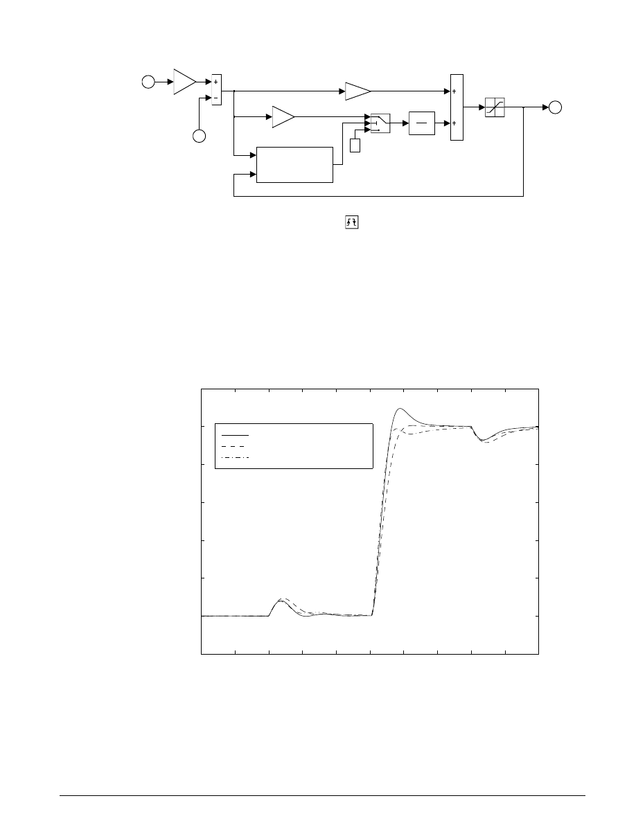
As is typical in the industry, the controller execution is synchronized with the engine’s crankshaft
rotation. The controller is embedded in a triggered subsystem that is triggered by the valve timing signal
described above. The detailed construction of the Controller subsystem is illustrated in Figure 1.5. Of note
is the use of the Discrete-Time Integrator block with its sample time parameter set (internally) at -1. This
indicates that the block should inherit its sample time, in this case executing each time the subsystem is
triggered. The key component that makes this a triggered subsystem is the Trigger block shown at the
bottom of Figure 1.5. Any subsystem can be converted to a triggered subsystem by dragging a copy of this
block into the subsystem diagram from the Simulink Connections library.
16
S
IMULINK
-S
TATEFLOW
T
ECHNICAL
E
XAMPLES
Triggered PI Controller
1
Throttle Setting
pi/30
rpm
to
rad/s
integrator input
controller output
enable integration
prevent windup
limit
output
Kp
Proportional Gain
Ki
Integral Gain
T
z -1
Discrete Time
Integrator
0
2 N
1
Desired
rpm
Figure 1.5: Speed Controller Subsystem
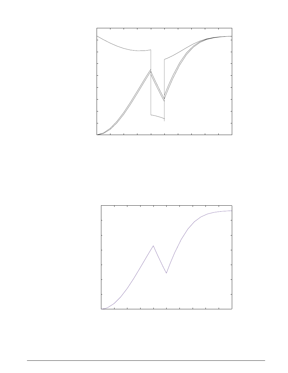
Results
Typical simulation results are shown in Figure 1.6. The speed set point steps from 2000 to 3000 RPM
at t = 5 sec. The torque disturbances are identical to those used in the previous example. Note the quick
transient response, with zero steady-state error.
Several alternative controller tunings are shown. These can be adjusted by the user at the M
ATLAB
command line. This allows the engineer to understand the relative effects of parameter variations.
0
1
2
3
4
5
6
7
8
9
10
1800
2000
2200
2400
2600
2800
3000
3200
time (Sec.)
engine speed (RPM)
Closed–Loop Engine Speed Control
Kp = 0.05, Ki = 0.1
Kp = 0.033, Ki = 0.064
Kp = 0.061, Ki = 0.072
Figure 1.6: Typical simulation results

U
SING
S
IMULINK AND
S
TATEFLOW IN
A
UTOMOTIVE
A
PPLICATIONS
17
Conclusions
The ability to model nonlinear, complex systems, such as the engine model described here, is one of
Simulink’s key features. The power of the simulation is evident in the presentation of the models above.
Simulink retains model fidelity, including precisely timed cylinder intake events, which is critical in
creating a model of this type. The two different models, the basic engine and complete speed control
system, demonstrate the flexibility of Simulink. In particular, the Simulink modeling approaches allow
rapid prototyping of an interrupt-driven engine speed controller.
References
1. P.R. Crossley and J.A. Cook, IEE International Conference ‘Control 91’, Conference Publication 332,
vol. 2, pp. 921-925, 25-28 March, 1991, Edinburgh, U.K.
2. The Simulink Model. Developed by Ken Butts, Ford Motor Company. Modified by Paul Barnard, Ted
Liefeld and Stan Quinn, The MathWorks, Inc., 1994-7.
3. J. J. Moskwa and J. K. Hedrick, "Automotive Engine Modeling for Real Time Control Application,"
Proc.1987 ACC, pp. 341-346.
4. B. K. Powell and J. A. Cook, "Nonlinear Low Frequency Phenomenological Engine Modeling and
Analysis," Proc. 1987 ACC, pp. 332-340.
5. R. W. Weeks and J. J. Moskwa, "Automotive Engine Modeling for Real-Time Control Using
Matlab/Simulink," 1995 SAE Intl. Cong. paper 950417.
18
S
IMULINK
-S
TATEFLOW
T
ECHNICAL
E
XAMPLES
II. A
NTI
-L
OCK
B
RAKING
S
YSTEM
Summary
This example describes a simple model for an Anti-Lock Braking System (ABS). The model
absbrake.mdl
simulates the dynamic behavior of a vehicle under hard braking conditions. The model
represents a single wheel, which may be replicated a number of times to create a model for a multi-wheel
vehicle. The Simulink block diagram is shown in Figure 2.1.
ABS Braking Model
Developed by Larry Michaels
The MathWorks, Inc
s
1
stopping distance
Double click
to run model
mu slip
friction curve
Kf
force &
torque
Wheel
Speed
m*g/4
Weight
s
1
Vehicle
speed
time
slp
yout
STOP
Rr
1.0 - u(1)/(u(2) + (u(2)==0)*eps)
Relative Slip
x
100
TB.s+1
Hydraulic Lag
0.2
Desired
relative
slip
ctrl
Brake
pressure
Bang bang
controller
1/Rr
1/I
-1/m
Ff
tire torque
brake torque
s
1
s
1
Figure 2.1: Simulation of the dynamic behavior of a vehicle under hard braking conditions
Analysis and
The wheel rotates with an initial velocity corresponding to the vehicle speed before the brakes are applied.
Physics
We used separate integrators to compute wheel speed and vehicle speed. The two speeds are used to
calculate slip, which is determined by
ω
ω
ω
v
v
r
w
v
V
R
slip
=
= −
/
1
Equation 2.1
where,
ω
ω
v
v
r
w
V
R
=
=
=
=
vehicle speed, in terms of the corresponding wheel angular velocity
vehicle linear velocity
wheel radius
wheel angular velocity
From these relationships we see that slip is 0 when wheel speed (
ω
w
) and the corresponding vehicle speed
(
ω
v
) are equal, and slip is 1 when the wheel is locked (
ω
w
= 0). A desirable slip value is 0.2, which means
that the number of wheel revolutions equals 0.8 times the number of revolutions under nonbraking

U
SING
S
IMULINK AND
S
TATEFLOW IN
A
UTOMOTIVE
A
PPLICATIONS
19
conditions with the same vehicle velocity. This maximizes the adhesion between the tire and road to
minimize the stopping distance with the available friction.
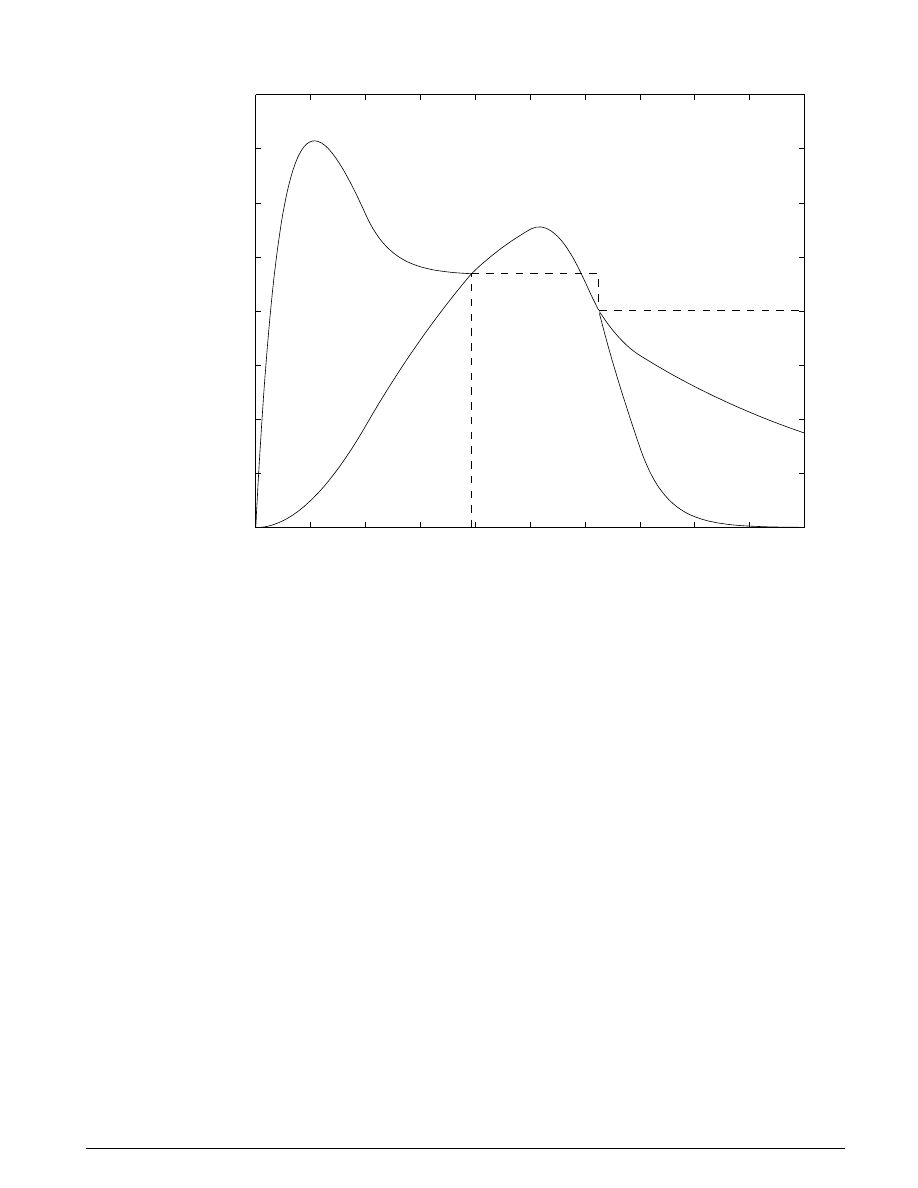
Modeling
The symbol
µ
, representing the friction coefficient between the tire and the road surface, is an empirical
function of slip, known as the
µ
-slip curve. We created
µ
-slip curves using M
ATLAB
variables that were
brought into the block diagram using a Simulink lookup table. The model multiplies the friction
coefficient,
µ
, by the weight on the wheel, W, to yield the frictional force, Ff , acting on the circumference of
the tire. Ff is divided by the vehicle mass to give the vehicle deceleration, which the model integrates to
obtain vehicle velocity. In this model, we used an ideal anti-lock braking controller, that uses “bang-
bang” control based upon the error between actual slip and desired slip. We set the desired slip to the
value of slip at which the
µ
-slip curve reaches a peak value, this being the optimum value for minimum
braking distance
1
.
By subtracting slip from desired slip, and feeding this signal into a bang-bang control (+1 or -1,
depending on the sign of the error), the model controls the rate of change of brake pressure. This on/off
rate passes through a first-order lag that represents the delay associated with the hydraulic lines of the
brake system. The model then integrates the filtered rate to yield the actual brake pressure. The resulting
signal, multiplied by the piston area and radius with respect to the wheel (Kf), is the brake torque applied
to the wheel. The model also multiplies the frictional force on the wheel by the wheel radius, R
r
, to give the
accelerating torque of the road surface on the wheel. The brake torque is subtracted to give the net torque
on the wheel. Dividing the net torque by the wheel rotational inertia, I, yields the wheel acceleration,
which is then integrated to provide wheel velocity. In order to prevent wheel speed and vehicle speed from
going negative, limited integrators are used in this model.
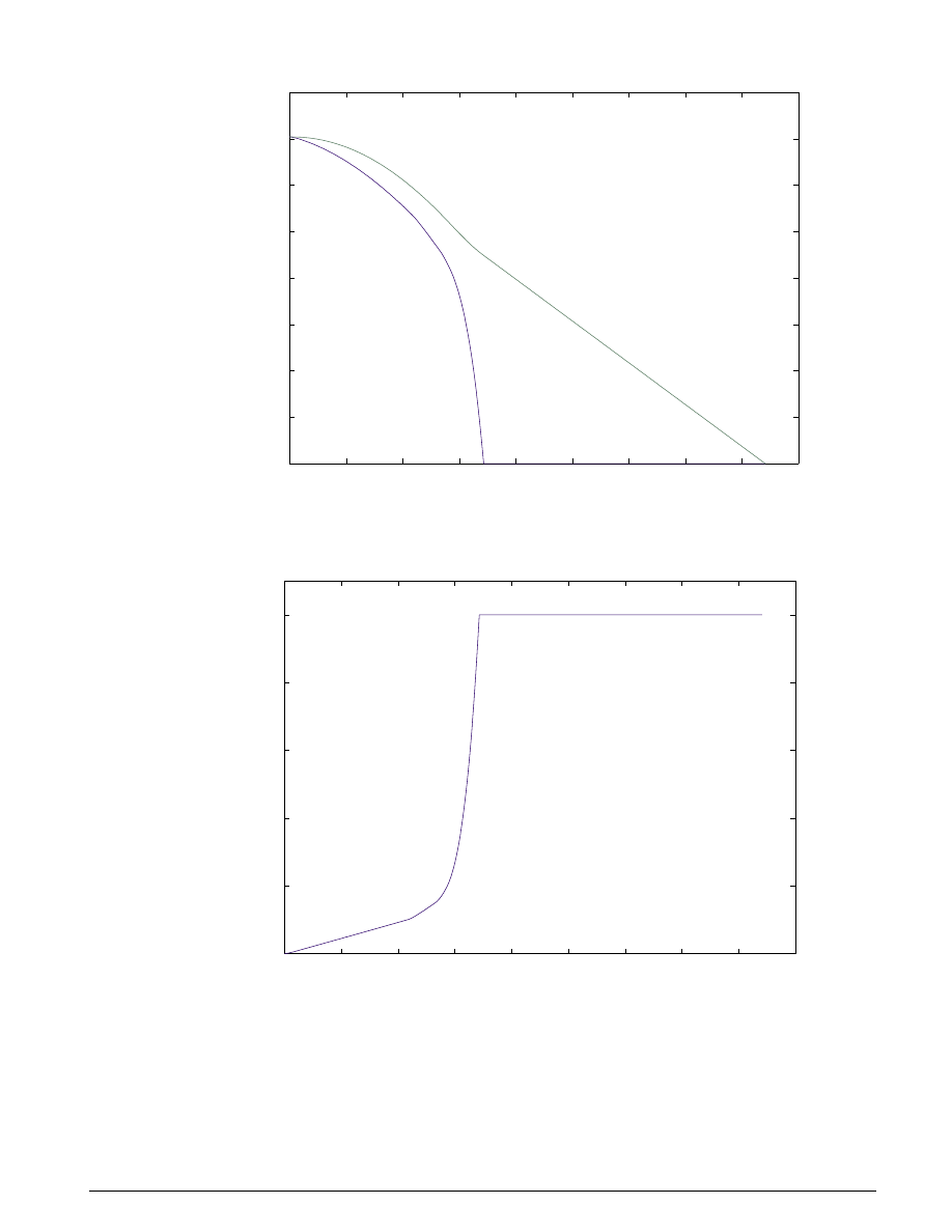
Results
Figure 2.2 and Figure 2.3 plot the results of a simulation run for a given set of parameters. Figure 2.2
shows the wheel angular velocity,
ω
w
, and corresponding vehicle angular velocity,
ω
v
, which shows that
ω
w
stays below
ω
v
without locking up, with vehicle speed going to zero in less than 15 seconds.
1
In an actual vehicle, slip cannot be measured directly, so this control algorithm is not practical. It was
used in this example to illustrate the conceptual construction of such a simulation model. The real
engineering value of a simulation like this is in demonstrating the potential of the control concept prior
to addressing the specific issues of implementation.
20
S
IMULINK
-S
TATEFLOW
T
ECHNICAL
E
XAMPLES
0
5
10
15
0
10
20
30
40
50
60
70
80
Vehicle speed and wheel speed
Speed(rad/sec)
Time(secs)
Vehicle speed (
ω
v
)
Wheel speed (
ω
w
)
Figure 2.2: Simulation showing the wheel and corresponding
vehicle angular velocities,
ω
w
and
ω
v
0
5
10
15
0
0.1
0.2
0.3
0.4
0.5
0.6
0.7
0.8
0.9
1
Slip
Time(secs)
Figure 2.3: Normalized wheel slip
To make the results more meaningful, consider the vehicle behavior without ABS. At the M
ATLAB
command line, set the model variable
ctrl = 0
. As can be seen in Figure 2.1, this disconnects the slip
feedback from the controller, resulting in maximum braking. The results are shown in Figures 2.4
and 2.5.
U
SING
S
IMULINK AND
S
TATEFLOW IN
A
UTOMOTIVE
A
PPLICATIONS
21
0
2
4
6
8
10
12
14
16
18
0
10
20
30
40
50
60
70
80
Vehicle speed (
ω
v
)
Wheel speed (
ω
ω
)
Vehicle speed and wheel speed
Time (secs)
Speed (rad/sec)
Figure 2.4: Wheel and corresponding vehicle angular velocities,
ω
w
and
ω
v
, without ABS
0
2
4
6
8
10
12
14
16
18
0
0.2
0.4
0.6
0.8
1
Normalized Slip
Time (secs)
Figure 2.5: Normalized wheel slip, without ABS
In Figure 2.4 observe that the wheel locks up in about seven seconds and the braking, from that point on,
is applied in a less-than-optimal part of the slip curve. That is, when slip = 1, as seen in Figure 2.5, the tire
is skidding so much on the pavement that the friction force between the two has dropped off.
22
S
IMULINK
-S
TATEFLOW
T
ECHNICAL
E
XAMPLES
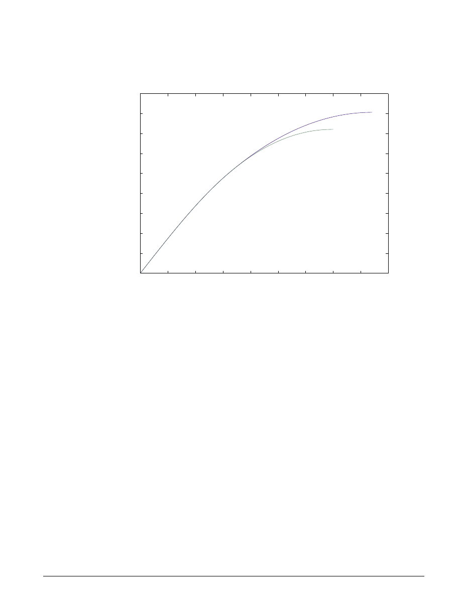
This is, perhaps, more meaningful in terms of the comparison shown in Figure 2.6. The distance traveled
by the vehicle is plotted for the two cases. Without ABS, the vehicle skids about an extra 100 feet, taking
about three seconds longer to come to a stop.
0
2
4
6
8
10
12
14
16
18
0
100
200
300
400
500
600
700
800
900
Hard Braking with and without ABS
Time (secs)
stopping distance (feet)
without ABS
with ABS
Figure 2.6: Simulated performance c omparison
Conclusions
This model demonstrates how Simulink can be used to simulate a braking system under the action of an
ABS controller. The controller in this example is idealized, but any proposed control algorithm can be
used in its place to evaluate the system’s performance.
The Real-Time Workshop may be used with Simulink as a valuable tool for rapid prototyping of the
proposed algorithm. C code is generated and compiled for the controller hardware to test the concept in a
vehicle. This significantly reduces the time needed to prove out new ideas by enabling actual testing early
in the development cycle.
For a hardware-in-the-loop braking system simulation, we would remove the bang-bang controller and
run the equations of motion on real-time hardware to emulate the wheel and vehicle dynamics. We
would do this by generating real-time C code for this model using the Real-Time Workshop. We could
then test an actual ABS controller by interfacing it to the real-time time hardware which would run the
generated code. In this scenario, the real-time model would send the wheel speed to the controller, and the
controller would send brake action to the model.
U
SING
S
IMULINK AND
S
TATEFLOW IN
A
UTOMOTIVE
A
PPLICATIONS
23
III.
C
LUTCH
E
NGAGEMENT
M
ODEL
Summary
This example demonstrates the use of Simulink to model and simulate a rotating clutch system.
Although modeling a clutch system is difficult because of topological changes in the system dynamics
during lockup, this example shows how Simulink’s enabled subsystems feature easily handles such
problems. We illustrate how to employ important Simulink modeling concepts in the creation of the
clutch simulation. Designers can apply these concepts to many models with strong discontinuities and
constraints that may change dynamically.
The clutch system in this example consists of two plates that transmit torque between the engine and
transmission. There are two distinct modes of operation: slipping, where the two plates have differing
angular velocities; and lockup, where the two plates rotate together. Handling the transition between these
two modes presents a modeling challenge. As the system loses a degree of freedom upon lockup, the
transmitted torque goes through a step discontinuity. The magnitude of the torque drops from the
maximum value supported by the friction capacity to a value that is necessary to keep the two halves of
the system spinning at the same rate. The reverse transition, break-apart, is likewise challenging, as the
torque transmitted by the clutch plates exceeds the friction capacity.
There are two methods for solving this type of problem:
1. Compute the clutch torque transmitted at all times, and employ this value directly in the model
2. Use two different dynamic models and switch between them at the appropriate times
Because of its overall capabilities, Simulink can model either method. In this example, we describe a
simulation for the second method. In the second method, switching between two dynamic models must
be performed with care to ensure that the initialized states of the new model match the state values
immediately prior to the switch. But, in either approach, Simulink facilitates accurate simulation due to
its ability to recognize the precise moments at which transitions between lockup and slipping occur.
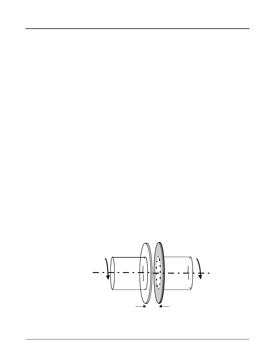
Analysis and
The clutch system was analyzed using a lumped-parameter model, according to the configuration shown
Physics
in Figure 3.1.
Figure 3.1: The clutch system, analyzed using a lumped-parameter model
I
e
I
v
F
n
ω
v
T
in
ω
e

24
S
IMULINK
-S
TATEFLOW
T
ECHNICAL
E
XAMPLES
The following variables are used in the analysis and modeling.
T
F
I I
b b
r r
R
T
T
in
n
e
v
e
v
k
s
e
v
c
=
=
=
=
=
=
=
=
=
=
input (engine) torque
normal force between friction plates
moments of inertia for the engine and for the transmission/vehicle
damping rates at theengine and transmission/vehicle sides of the clutch
kinetic and static coefficients of friction
,
angular speeds of the engine and transmission input shafts
inner and outer radii of the clutch plate friction surfaces
equivalent net radius
torque transmitted through the clutch
friction torque required of the clutch to maintain lockup
,
,
,
,
µ µ
ω ω
1
2
1
1
The state equations for the coupled system are derived as follows:
I
T
b
T
I
T
b
e
e
in
e
e
cl
v
v
cl
v v
˙
˙
ω
ω
ω
ω
=
−
−
=
−
Equation 3.1
The torque capacity of the clutch is a function of its size, friction characteristics, and the normal force that
is applied.
T
A
da
F
r
r
r drd
RF
R
r
r
r
r
f
A
n
r
r
n
max
(
)
,
(
)
(
)
=
×
=
−
=
=
−
−
∫∫
∫
∫
r
F
f
µ
π
θ
µ
π
2
2
1
2
2
0
2
2
3
2
3
1
3
2
2
1
2
1
2
When the clutch is slipping, the model uses the kinetic coefficient of friction and the full capacity is
available, in the direction that opposes slip.
T
RF
T
T
fmaxk
n
k
cl
e
v
fmaxk
=
=
−
2
3
µ
ω
ω
sgn(
)
Equation 3.3
When the clutch is locked,
ω
e
=
ω
v
=
ω
and the system torque acts on the combined inertia as a single
unit. So, we combine the differential equations (Equation 3.1) into a single equation for the locked state.
(
) ˙
(
)
I
I
T
b
b
e
v
in
e
v
+
=
−
+
ω
ω
Equation 3.4
Solving (Equation 3.1) and (Equation 3.4), the torque transmitted by the clutch while locked is:
Equation 3.2
U
SING
S
IMULINK AND
S
TATEFLOW IN
A
UTOMOTIVE
A
PPLICATIONS
25
T
T
I T
I b
I b
I
I
cl
f
v
in
v e
e v
v
e
=
=
−
−
+
(
)
ω
Equation 3.5
The clutch thus remains locked unless the magnitude of T
f
exceeds the static friction capacity, T
fmaxs
, where
T
RF
fmaxs
n
s
=
2
3
µ
Equation 3.6
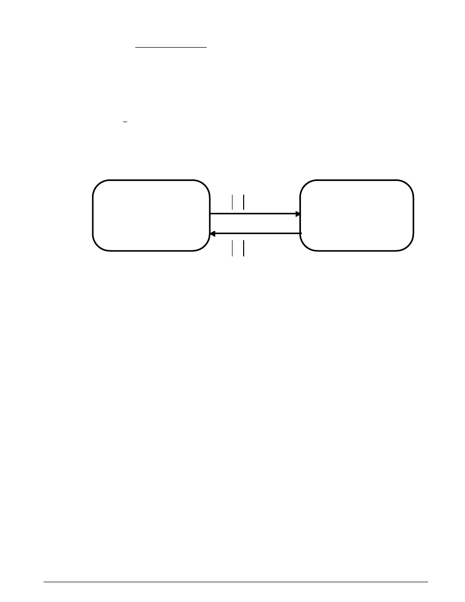
A state diagram describes the overall behavior.
Figure 3.2: A state diagram describing the friction mode transitions
Modeling
The simulation model for the clutch system (
clutch.mdl
) makes use of enabled subsystems, a
particularly useful feature in Simulink. The simulation can use one subsystem while the clutch is
slipping and the other when it is locked. A diagram of the Simulink model appears in Figure 3.3.
Locked
(
) ˙
(
)
I
I
T
b
b
T
T
e
v
in
e
v
v
e
cl
f
+
=
−
+
=
=
=
ω
ω
ω
ω
ω
ω
ω
e
v
f
fmaxs
and
T
T
=
≤
T
T
f
fmaxs
>
Slipping
I
T
b
T
I
T
b
T
T
e
e
in
e
e
cl
v
v
cl
v v
cl
e
v
fmaxk
˙
˙
sgn(
)
ω
ω
ω
ω
ω
ω
=
−
−
=
−
=
−
26
S
IMULINK
-S
TATEFLOW
T
ECHNICAL
E
XAMPLES
Clutch Model in Simulink 2
A Demonstration of Enabled Subsystems
8
Max Static Friction Torque
7
FrictionTorque
Required
for Lockup
6
BreakApart
Flag
5
Lockup
Flag
4
Locked
Flag
3
w
2
wv
1
we
Tfmaxk
Tin
we
wv
Unlocked
Tin
w
Locked
Tin
Tfmaxs
locked
lock
unlock
Tf
Friction Mode Logic
Fn
Tfmaxk
Tfmaxs
Friction
Model
Tin
Engine
Torque
Fn
Clutch
Pedal
clutch unlocked
clutch locked
Figure 3.3: The top level S imulink model
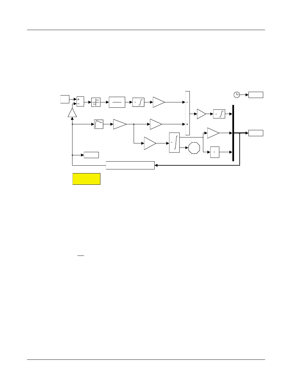
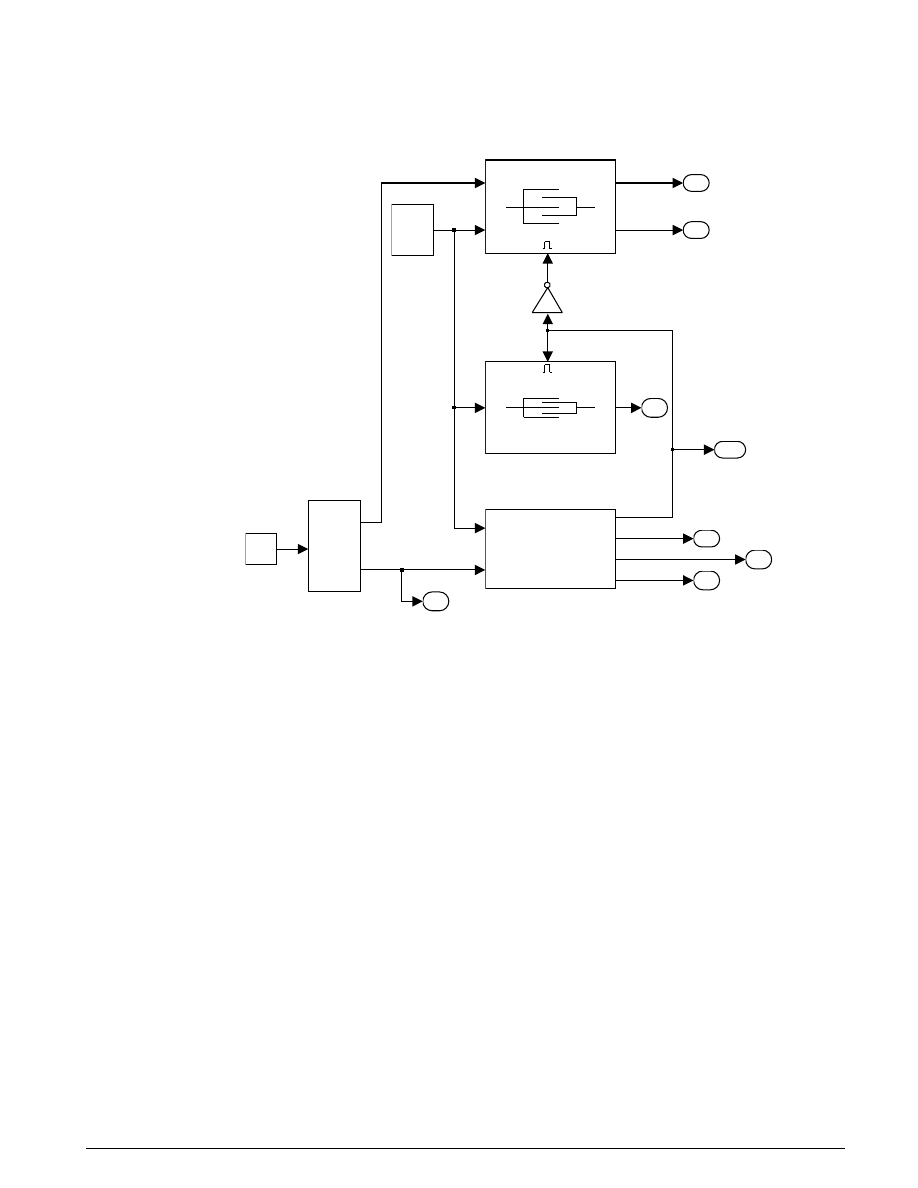
The first subsystem,
Unlocked
, models both sides of the clutch, coupled by the friction torque. It is
constructed around the integrator blocks which represent the two speeds, as shown in Figure 3.4. The
model uses gain, multiplication, and summation blocks to compute the speed derivatives (acceleration)
from the states and the subsystem inputs of engine torque, Tin, and clutch capacity, Tfmaxk.
Enabled subsystems, such as Unlocked, feature several other noteworthy characteristics. The Enable
block at the top of the diagram in Figure 3.4 defines the model as an enabled subsystem. To create an
enabled subsystem, we group the blocks together like any other subsystem. We then insert an Enable
block from the Simulink Connections library. This means that:
1.
An enable input appears on the subsystem block, identified by the pulse-shaped symbol used on the
Enable block itself.
2.
The subsystem executes only when the signal at the enable input is greater than zero.
In this example, the Unlocked subsystem executes only when the supervising system logic determines
that it should be enabled.
U
SING
S
IMULINK AND
S
TATEFLOW IN
A
UTOMOTIVE
A
PPLICATIONS
27
2
wv
1
we
[locked_w]
w0
[locked_w]
w0
W_Sum
s
1
Vehicle
Integrator
1/Iv
Vehicle
Inertia
bv
Vehicle
Damping
V_Sum
Sign
Max
Dynamic
Friction
Torque
unlocked_wv
unlocked_we
s
1
Engine
Integrator
1/Ie
Engine
Inertia
be
Engine
Damping
E_Sum
Enable
2
Tin
1
Tfmaxk
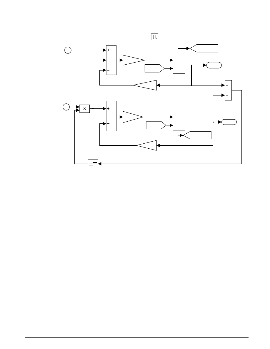
Figure 3.4: The Unlocked subsystem
There is another important consideration when using systems that can be enabled or disabled. When the
system is enabled, the simulation must reinitialize the integrators to begin simulating from the correct
point. In this case, both sides of the clutch are moving at the same velocity the moment it unlocks. The
Unlocked subsystem, which had been dormant, needs to initialize both integrators at that speed in order
to keep the system speeds continuous.
The simulation uses From blocks to communicate the state of the locked speed to the initial condition
inputs of the two integrators. Each From block represents an invisible connection between itself and a
Goto block somewhere else in the system. The Goto blocks connect to the state ports of the integrators so
that the model can use these states elsewhere in the system without explicitly drawing in the connecting
lines.
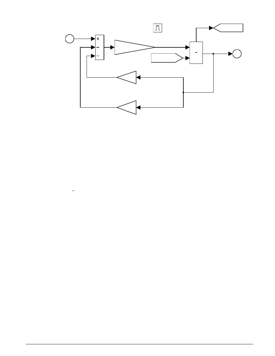
The other enabled block seen in the top-level block diagram is the Locked subsystem, shown in Figure 3.5.
This model uses a single state to represent the engine and vehicle speeds. It computes acceleration as a
function of the speed and input torque. As in the Unlocked case, a From block provides the integrator
initial conditions and a Goto block broadcasts the state for use elsewhere in the model. While simulating,
either the Locked or the Unlocked subsystem is active at all times. Whenever the control changes, the
states are neatly handed off between the two.
28
S
IMULINK
-S
TATEFLOW
T
ECHNICAL
E
XAMPLES
1
w
[unlocked_we]
w0
bv
Vehicle
Damping
1/(Iv+Ie)
Inertia
locked_w
s
1
Engine/Vehicle
Integrator
be
Engine
Damping
Enable
1
Tin
Omega
Omega
Omega
Figure 3.5: The Locked subsystem
The simulation uses other blocks in the system to calculate the friction capacity and to supply the logic
that determines which of the Locked or Unlocked subsystems should be enabled.
The Friction Model subsystem computes the static and kinetic friction according to Equation 3.7, with the
appropriate friction coefficient.
T
RF
fmax
n
=
2
3
µ
Equation 3.7
The remaining blocks calculate the torque required for lockup (Equation 3.5), and implement the logic
described in Figure 3.2. One key element is located in the Lockup Detection subsystem within the Friction
Mode Logic subsystem. This is the Simulink Hit Crossing block which precisely locates the instant at
which the clutch slip reaches zero. This places the mode transition at exactly the right moment.
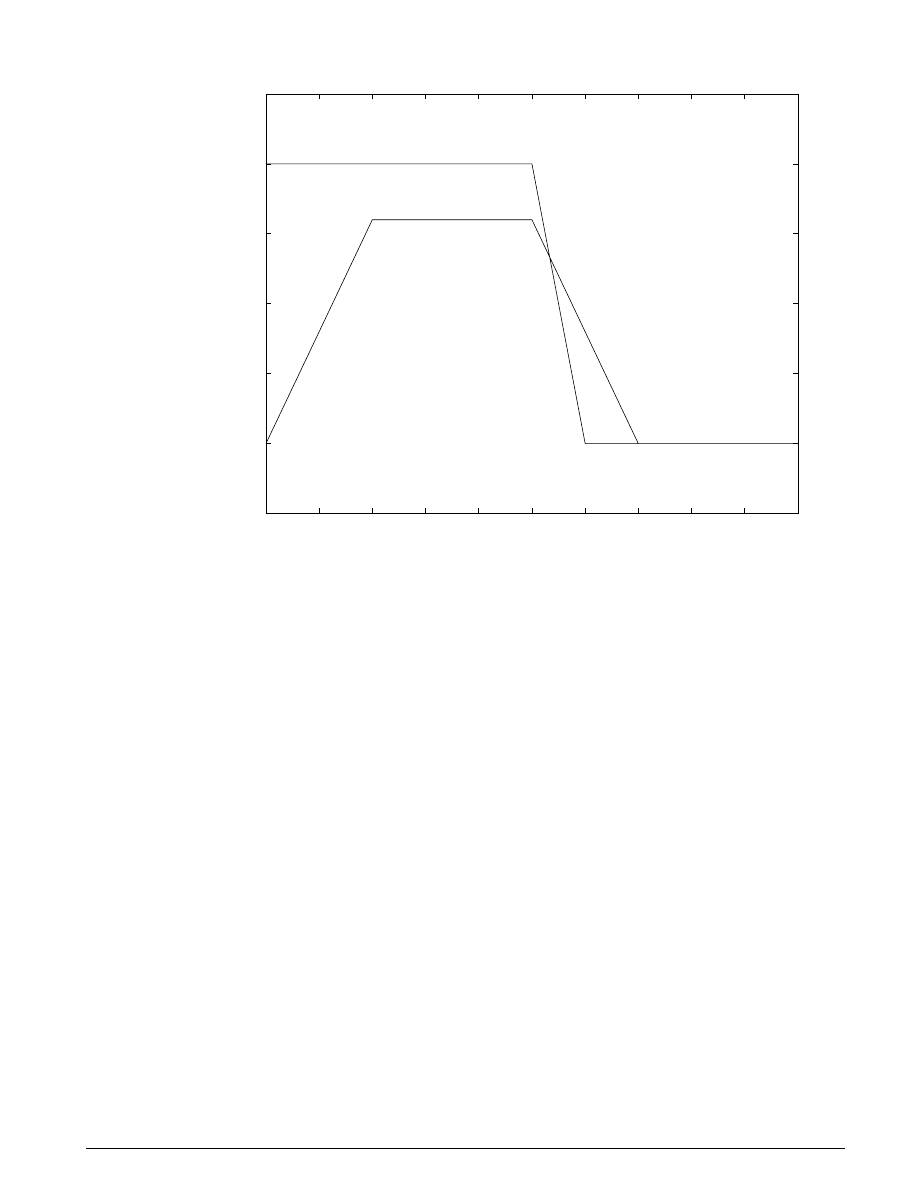
The system inputs are normal force, F
n
, and engine torque, T
in
. Each of these is represented by a matrix
table in the M
ATLAB
workspace and plotted in Figure 3.6 below. The Simulink model incorporates these
inputs by using From Workspace blocks.
U
SING
S
IMULINK AND
S
TATEFLOW IN
A
UTOMOTIVE
A
PPLICATIONS
29
0
1
2
3
4
5
6
7
8
9
10
-0.5
0
0.5
1
1.5
2
2.5
time (sec)
Engine Torque and Clutch Normal Force
Clutch Example Default Inputs
T
in
F
n
Figure 3.6: System inputs of normal force and engine torque
Results
The following parameter values are used to demonstrate the simulation. These are not meant to represent
the physical quantities corresponding to an actual system, but rather to facilitate a meaningful baseline
demonstration.
I
I
b
b
R=
e
v
e
v
k
s
=
−
=
−
=
=
=
=
1 kg m
5 kg m
2 Nm/rad/sec
1 Nm/rad/sec
1
1.5
m
2
2
µ
µ
1
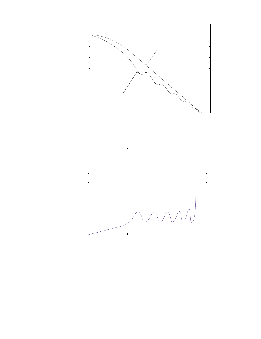
For the inputs shown above, the system velocities behave as shown in Figure 3.7 below. The simulation
begins in the Unlocked mode, with an initial engine speed flare as the vehicle side accelerates its larger
inertia. At about t = 4 seconds, the velocities come together and remain locked, indicating that the clutch
capacity is sufficient to transmit the torque. At t = 5, the engine torque begins to decrease, as does the
normal force on the friction plates. Consequently, the onset of slip occurs at about t = 6.25 seconds as
indicated by the separation of the engine and vehicle speeds.
30
S
IMULINK
-S
TATEFLOW
T
ECHNICAL
E
XAMPLES
0
1
2
3
4
5
6
7
8
9
10
0
0.1
0.2
0.3
0.4
0.5
0.6
0.7
0.8
time (sec)
shaft speeds (rad/sec)
Baseline Clutch Performance
ω
e
ω
e
ω
v
ω
v
ω
Figure 3.7: Behavior of the system velocities
Notice that the various states remain constant while they are disabled. At the time instants at which
transitions take place, the state handoff is both continuous and smooth. This is a result of supplying each
integrator with the appropriate initial conditions to use when the state is enabled.
Conclusions
This example shows how to use Simulink and its standard block library to model, simulate, and analyze a
system with topological discontinuities. This is a powerful demonstration of the Hit Crossing block and
how it can be used to capture specific events during a simulation. The Simulink model of this clutch
system can serve as a guide when creating models with similar characteristics. In any system with
topological discontinuities, the principles used in this example may be applied.
U
SING
S
IMULINK AND
S
TATEFLOW IN
A
UTOMOTIVE
A
PPLICATIONS
31
IV. S
USPENSION
S
YSTEM
Summary
This example describes a simplified half-car model (
suspn.mdl
) that includes an independent front and
rear vertical suspension as well as body pitch and bounce degrees of freedom. We provide a description of
the model to show how simulation can be used for investigating ride and handling characteristics. In
conjunction with a powertrain simulation, the model could investigate longitudinal shuffle resulting
from changes in throttle setting.
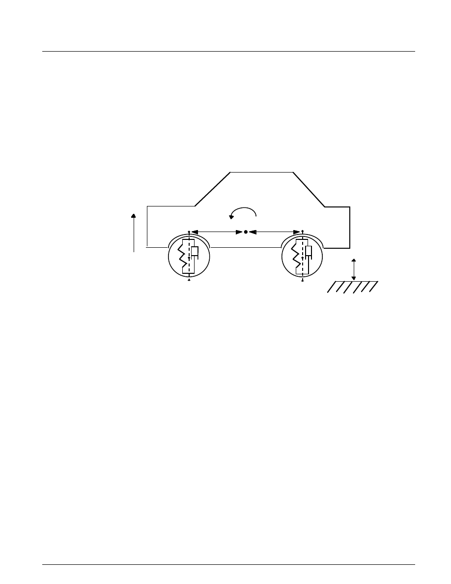
Analysis and
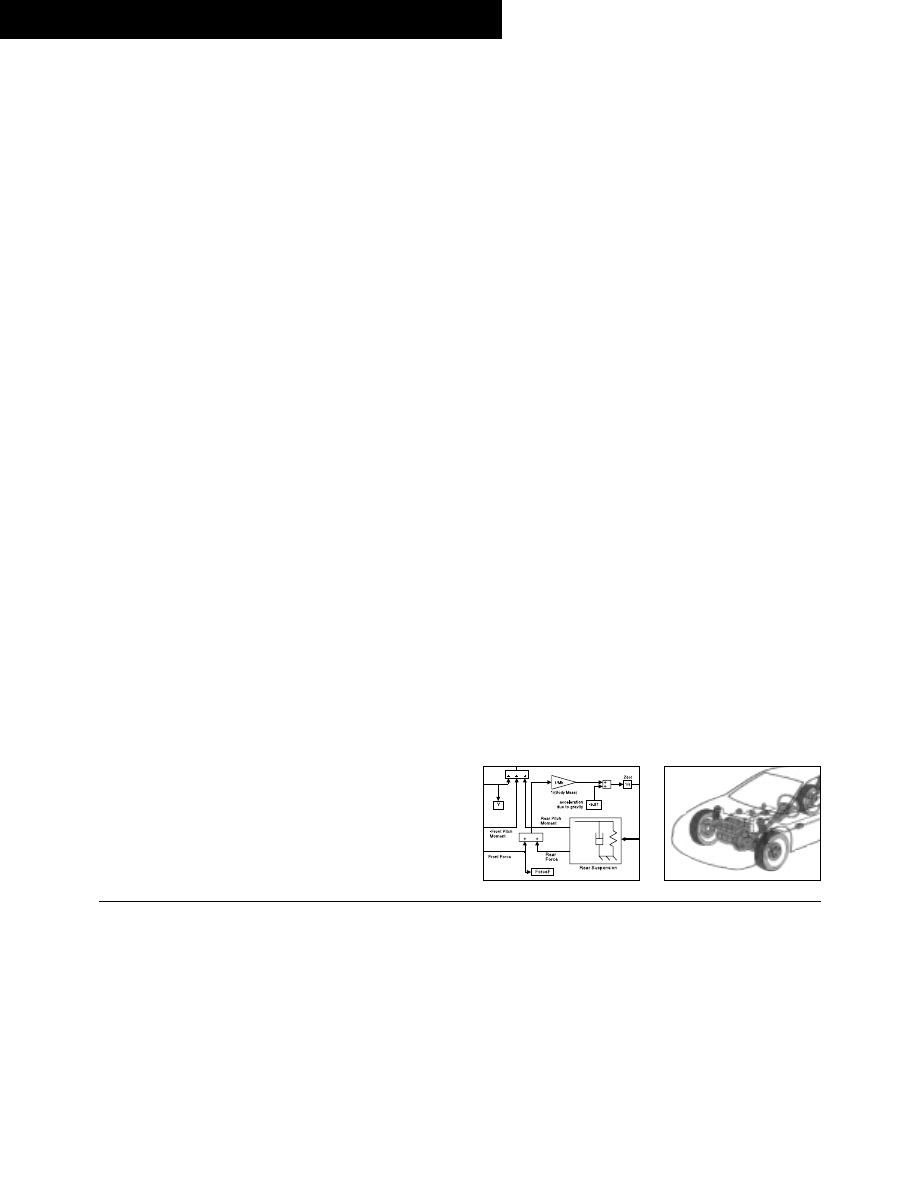
The diagram in Figure 4.1 illustrates the modeled characteristics.
Physics
Figure 4.1: A free-body diagram of the half-car model
In this example, we model the front and rear suspension as spring/damper systems. A more detailed
model would include a tire model as well as damper nonlinearities such as velocity-dependent damping
with greater damping during rebound than compression. The vehicle body has pitch and bounce degrees
of freedom, which are represented in the model by four states: vertical displacement, vertical velocity, pitch
angular displacement, and pitch angular velocity. A full six degrees of freedom model can be implemented
using vector algebra blocks to perform axis transformations and force/displacement/velocity calculations.
The front suspension influences the bounce, or vertical degree of freedom, according to the relationships
in Equation 4.1.
F
K
L
z
C
L
z
F
K
C
L
z z
front
f
f
f
f
front
f
f
f
=
−
+
−
=
=
=
=
=
2
2
(
)
(
˙
˙ ),
,
˙
, ˙
θ
θ
θ θ
upward force on body from front suspension
suspension spring rate and damping rate at each wheel
horizontal distance from body center of gravity to front suspension
,
pitch (rotational) angle and rate of change
bounce (vertical) distance and velocity
Equation 4.1
K
f
C
f
K
r
C
r
L
f
L
r
C of G
Z
θ
h
32
S
IMULINK
-S
TATEFLOW
T
ECHNICAL
E
XAMPLES
The pitch contribution of the front suspension follows directly.
M
L F
front
f
front
= −
=
,
pitch moment due to front suspension
Equation
4.2
Similarly, for the rear suspension:
F
K L
z
C L
z
F
K C
L
M
L F
M
rear
r
r
r
r
rear
r
r
r
rear
r rear
rear
= −
+
−
+
=
=
=
=
=
2
2
(
)
(
˙
˙ ),
,
,
θ
θ
upward force on body from rear suspension
suspension spring rate and damping rate at each wheel
horizontal distance from body center of gravity to rear suspension
pitch moment due to rear suspension
Equation
4.3
The forces and moments result in body motion according to Newton.
M z
F
F
M g
M
g
I
M
M
M
I
M
b
front
rear
b
b
yy
front
rear
y
yy
y
˙˙
,
˙˙
,
=
+
−
=
=
=
+
+
=
=
body mass
gravitational acceleration
body moment of inertia about center of gravity
moment introduced by vehicle acceleration
θ
Equation
4.4
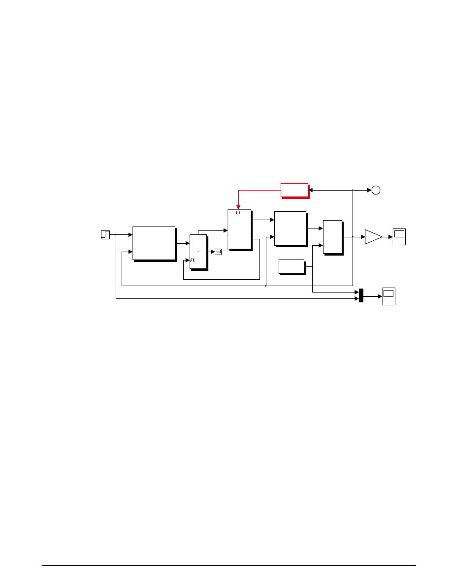
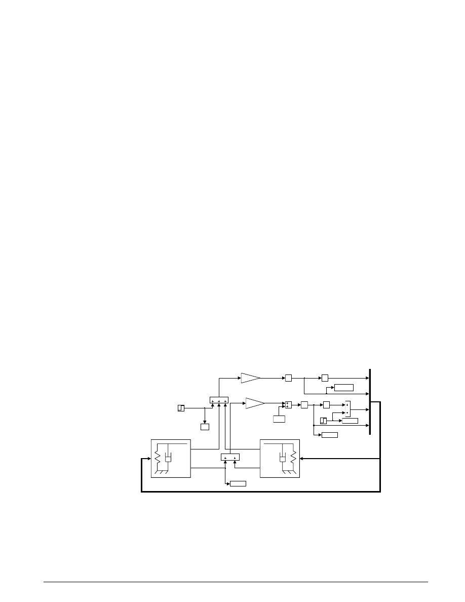
Modeling
We saved the Simulink suspension model as
suspn.mdl
and opened it by typing
suspn
at the M
ATLAB
prompt.
Vehicle Suspension Model
Developed by David Maclay
Cambridge Control, Ltd.
rev. 8/20/97, SQ
-9.81
acceleration
due to gravity
1/s
Zdot
1/s
Z
Zdot
h
THETAdot
Y
ForceF
1/s
THETAdot
1/s
THETA
Road
Height
Rear Suspension
Mu
Moment
due to longitudinal
vehicle acceleration
Front Suspension
1/Mb
1/(Body Mass)
1/Iyy
1/(Body Inertia)
Rear Force
Rear Pitch Moment
-Front Pitch Moment
Front Force
THETA, THETAdot, Z, Zdot
4.2: The Simulink two degree of freedom suspension model
U
SING
S
IMULINK AND
S
TATEFLOW IN
A
UTOMOTIVE
A
PPLICATIONS
33
There are two inputs to the Vehicle Suspension model shown in Figure 4.2. The first input is the road
height. A step input here corresponds to the vehicle driving over a road surface with a step change in
height. The second input is a horizontal force acting through the center of the wheels that results from
braking or acceleration maneuvers. Since the longitudinal body motion is not modeled, this input
appears only as a moment about the pitch axis.
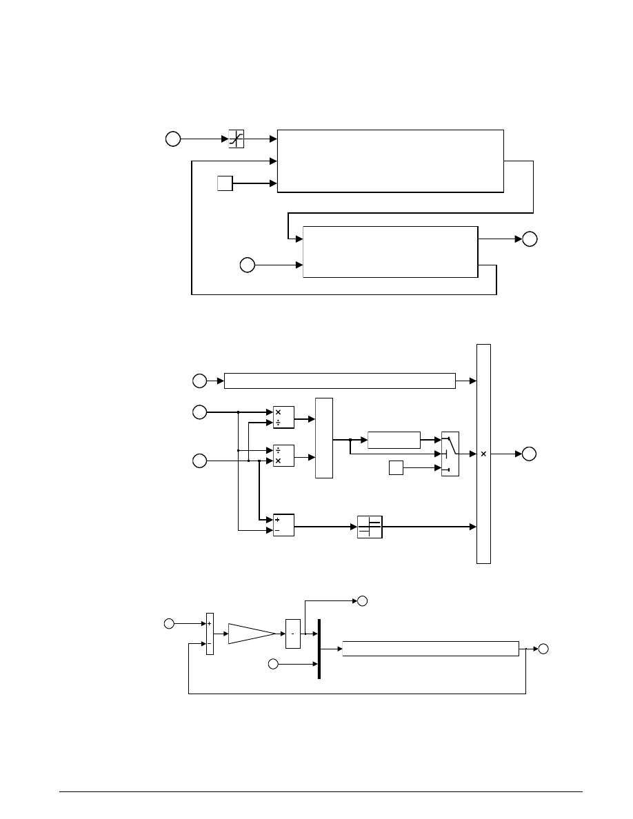
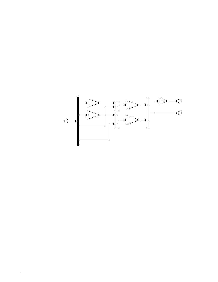
The spring/damper subsystem that models the front and rear suspensions is shown in Figure 4.3. The
block is used to model Equation 4.1 through 4.3. The equations are implemented directly in the Simulink
diagram through the straightforward use of Gain and Summation blocks. The differences between front
and rear are accounted for as follows. Because the subsystem is a masked block, a different data set (L, K
and C) can be entered for each instance. Furthermore, L is thought of as the Cartesian coordinate x, being
negative or positive with respect to the origin, or center of gravity. Thus, K
f
, C
f
and -L
f
are used for the
front and K
r
, C
r
and L
r
for the rear.
Two DOF Spring/Damper Model
2
Vertical
Force
1
pitch
Torque
2*K
stiffness
2*C
damping
L
MomentArm3
L
MomentArm2
L
MomentArm1
Fz
em
1
THETA
THETAdot
Z
Zdot
Figure 4.3: The Spring/Damper suspension subsystem
Results
To run this model, first set up the required parameters in the M
ATLAB
workspace. Run the following
M-file by typing
suspdat
, or from the M
ATLAB
command line, enter the data by typing:
Lf = 0.9;
% front hub displacement from body CG
Lr = 1.2; % rear hub displacement from body CG
Mb = 1200; % body mass in kg
Iyy = 2100;
% body moment of inertia about y-axis in kgm^2
kf = 28000; % front suspension stiffness in N/m
kr = 21000;
% rear suspension stiffness in N/m
cf = 2500;
% front suspension damping in N/(m/s)
cr = 2000;
% rear suspension damping in N/(m/s)
To run the simulation, select Start from the Simulink Simulation menu or type the following at the
M
ATLAB
command line:
[t,x] = sim('suspn2',10); % run a time response
34
S
IMULINK
-S
TATEFLOW
T
ECHNICAL
E
XAMPLES
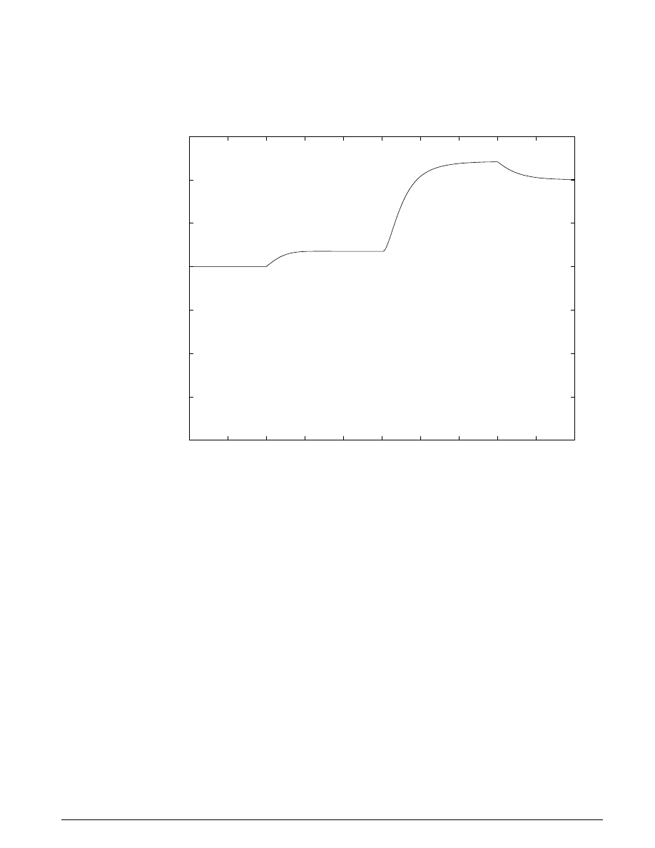
Figure 4.4 shows the plotted output results. You can automate setting the parameters, running the
simulation, and plotting these graphs by typing
suspgrph
at the M
ATLAB
command line prompt.
-5
0
5
x 10
-3
THETAdot
d
θ
/dt
Vehicle Suspension Model Simulation
-0.1
0
0.1
Zdot
dz/dt
6000
6500
7000
Ff
reaction force at front wheels
-5
0
5
10
15
x 10
-3
h
road height
0
1
2
3
4
5
6
7
8
9
10
0
50
100
Y
moment due to vehicle accel/decel
time in seconds
Figure 4.4: A summary of the suspension simulation output results
Conclusions
The Vehicle Suspension model allows you to simulate the effects of changing the suspension damping
and stiffness, thereby investigating the tradeoff between comfort and performance. In general, a racing
car has very stiff springs with a high damping factor, whereas a passenger vehicle designed for comfort
has softer springs and a more oscillatory response.
U
SING
S
IMULINK AND
S
TATEFLOW IN
A
UTOMOTIVE
A
PPLICATIONS
35
V.
H
YDRAULIC
S
YSTEMS
Summary
This example considers several hydraulic systems. The general concepts apply to suspension, brake,
steering, and transmission systems. We model three variations of systems employing pumps, valves, and
cylinder/piston actuators. The first features a single hydraulic cylinder which we develop, simulate and
save as a library block. In the next model, we use four instances of this block, as in an active suspension
system. In the final model, we model the interconnection of two hydraulic actuators, held together by a
rigid rod which supports a large mass.
In some cases we treat relatively small volumes of fluid as incompressible. This results in a system of
differential-algebraic equations (DAEs). Simulink solvers are well-suited to handle this type of problem
efficiently. The masking and library reference capabilities add extra power and flexibility. The creation of
custom blocks enables the implementation of important subsystems with user-defined parameter sets.
The Simulink library keeps a master version of these blocks so that models using a master block
automatically incorporate any revisions and refinements made to it.
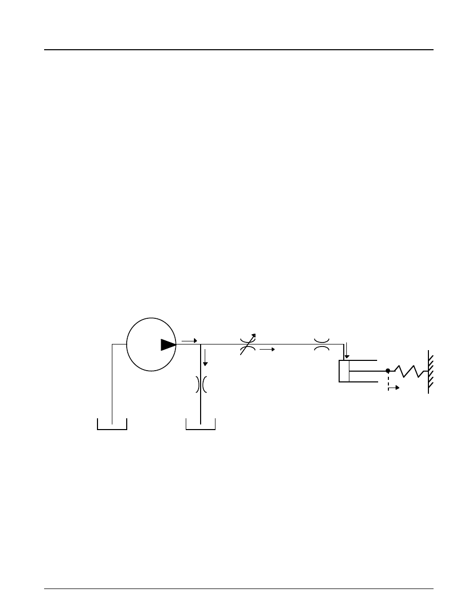
Analysis and
Figure 5.1 shows a schematic diagram of the basic model. The model directs the pump flow Q to
Physics
supply pressure p
1
from which laminar flow q1ex leaks to exhaust. The control valve for the
piston/cylinder assembly is modeled as turbulent flow through a variable-area orifice. Its flow q
12
leads to
intermediate pressure p
2
which undergoes a subsequent pressure drop in the line connecting it to the
actuator cylinder. The cylinder pressure p
3
moves the piston against a spring load, resulting in position x.
q
12
q
1ex
p
1
p
2
C
2
C
1
x
p
3
v
3
A
Q
q
23
Figure 5.1: Schematic diagram of the basic hydraulic system
At the pump output, the flow is split between leakage and flow to the control valve. The leakage, q
1ex
is
modeled as laminar flow.
pump
control valve
cylinder

36
S
IMULINK
-S
TATEFLOW
T
ECHNICAL
E
XAMPLES
Q
q
q
q
C p
p
Q
q
C
Q
q
q
C
p
ex
ex
ex
=
+
=
=
−
=
=
=
=
=
12
1
1
2 1
1
12
2
12
1
2
1
(
) /
pump flow
control valve flow
leakage
flow coefficient
pump pressure
Equation 5.1
We modeled turbulent flow through the control valve with the orifice equation. The sign and absolute
value functions accommodate flow in either direction.
q
C A
p
p
p
p
C
A
p
d
d
12
1
2
1
2
2
2
=
−
−
=
=
=
=
sgn(
)
ρ
ρ
orifice discharge coefficient
orifice area
pressure downstream of control valve
fluid density
Equation 5.2
The fluid within the cylinder pressurizes due to this flow, q
12
= q
23
, less the compliance of the piston
motion. We also modeled fluid compressibility in this case.
˙
˙
p
v
q
xA
p
v
p
V
A x
A
V
x
c
c
c
3
3
12
3
3
3
30
30
0
=
−
(
)
=
=
=
=
+
=
=
=
β
β
piston pressure
fluid bulk modulus
fluid volume at
cylinder cross – sectional area
fluid volume at
Equation 5.3
We neglected the piston and spring masses due to the large hydraulic forces. Force balance at the piston
gives:
x
p A
K
K
c
=
=
3
/
spring rate
Equation 5.4
cylinder cross–sectional area
U
SING
S
IMULINK AND
S
TATEFLOW IN
A
UTOMOTIVE
A
PPLICATIONS
37
We complete the system of equations by differentiating this relationship and incorporating the pressure
drop between p
2
and p
3
. The latter models laminar flow in the line from the valve to the actuator.
˙
˙
/
(
)
/
x
p A
K
q
q
C
p
p
p
p
q
C
C
c
=
=
=
−
=
+
=
3
23
12
1
2
3
2
3
12
1
1
laminar flow coefficient
Equation 5.5
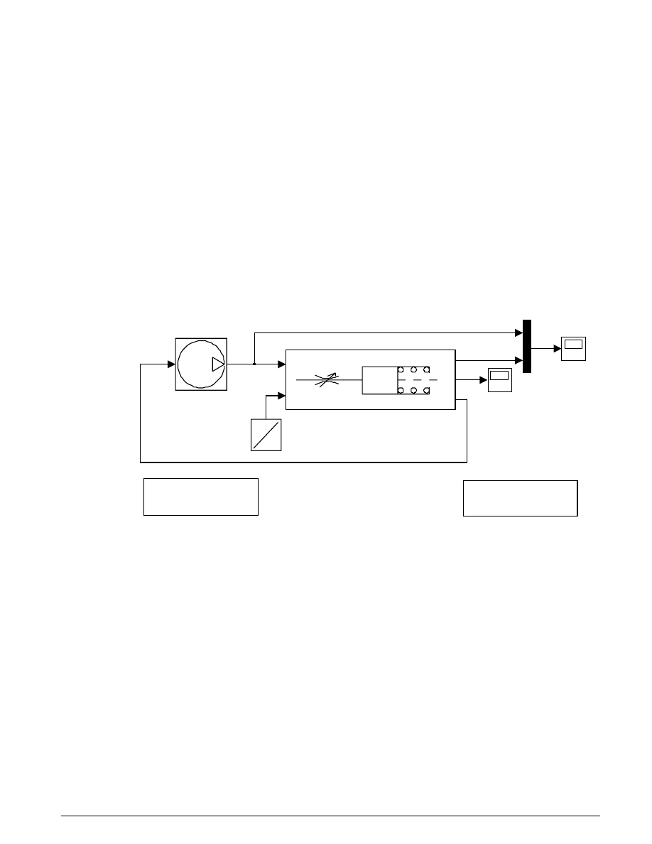
Modeling
Figure 5.2 shows the basic model, stored in the file
hydcyl.mdl
. Simulation inputs are the pump
flow and the control valve orifice area. The model is organized as two subsystems — the pump and the
actuator assembly.
Hydraulic Cylinder Model
p1
A
p
x
qin
valve/cylinder/piston/spring assembly
pump
pressures
p1 (yellow)
p2 (purple)
p3 (blue)
Mux
piston position
control valve
orifice area
Double click to run the
Simulation for 0.1 seconds
Double click to see
a 4 cylinder model.
Qout
p1
Figure 5.2: The basic pump/valve/actuator model
Pump
The pump model computes the supply pressure as a function of the pump flow and the load (output) flow
(Figure 5.3). A
From Workspace
block provides the pump flow data, Qpump. This is specified by a matrix
with column vectors of time points and the corresponding flow rates [T, Q]. The model subtracts the
output flow, using the difference, the leakage flow, to determine the pressure p
1
, as indicated above in
Equation 5.1. Since Qout = q
12
is a direct function of p
1
(via the control valve), this forms an algebraic
loop. An estimate of the initial value, p
10
, enables a more efficient solution.
We mask the subsystem in Simulink to facilitate ready access to the parameters by the user. The
parameters to be specified are T, Q, p
10
and the leakage flow coefficient, C
2
. For easy identification, we then
assigned the masked block the icon shown in Figure 5.2, and saved it in the Simulink library
hydlib.mdl
.
38
S
IMULINK
-S
TATEFLOW
T
ECHNICAL
E
XAMPLES
1
p1
1/C2
leakage
[T,Q]
Qpump
[p10]
IC
1
Qout
Figure 5.3: Hydraulic Pump Subsystem
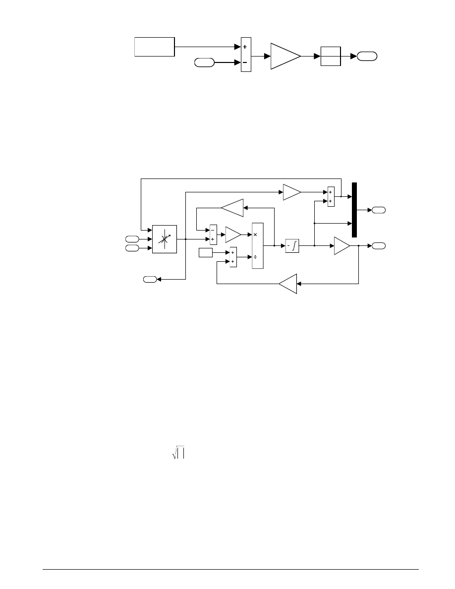
Actuator Assembly
valve/cylinder/piston/spring assembly
3
qin
2
x
1
p
s
1
piston
pressure
Mux
p2, p3
1/C1
laminar flow
pressure drop
Ac/K
force/spring
cylinder
volume
p2
Area
p1
q12
control valve
flow
beta
Ac
Ac^2/K
V30
2
A
1
p1
xdotAc
p3
p2
Figure 5.4: Hydraulic Actuator Subsystem
In Figure 5.4, a system of differential-algebraic equations models the cylinder pressurization with the
pressure
p
3
, which appears as a derivative in Equation 5.3 and is used as the state (integrator). If we
neglect mass, the spring force and piston position are direct multiples of p
3
and the velocity is a direct
multiple of
˙
p
3
. This latter relationship forms an algebraic loop around the bulk modulus Gain block,
Beta
. The intermediate pressure p
2
is the sum of p
3
and the pressure drop due to the flow from the valve to
the cylinder (Equation 5.5). This relationship also imposes an algebraic constraint through the control
valve and the 1/C1 gain.
The control valve subsystem computes the orifice (equation 5.2), with the upstream and downstream
pressures as inputs, as well as the variable orifice area. A lower level subsystem computes the “signed
square root,”
y
(u) u
=
sgn
. Three nonlinear functions are used, two of which are discontinuous. In
combination, however, y is a continuous function of u.

U
SING
S
IMULINK AND
S
TATEFLOW IN
A
UTOMOTIVE
A
PPLICATIONS
39
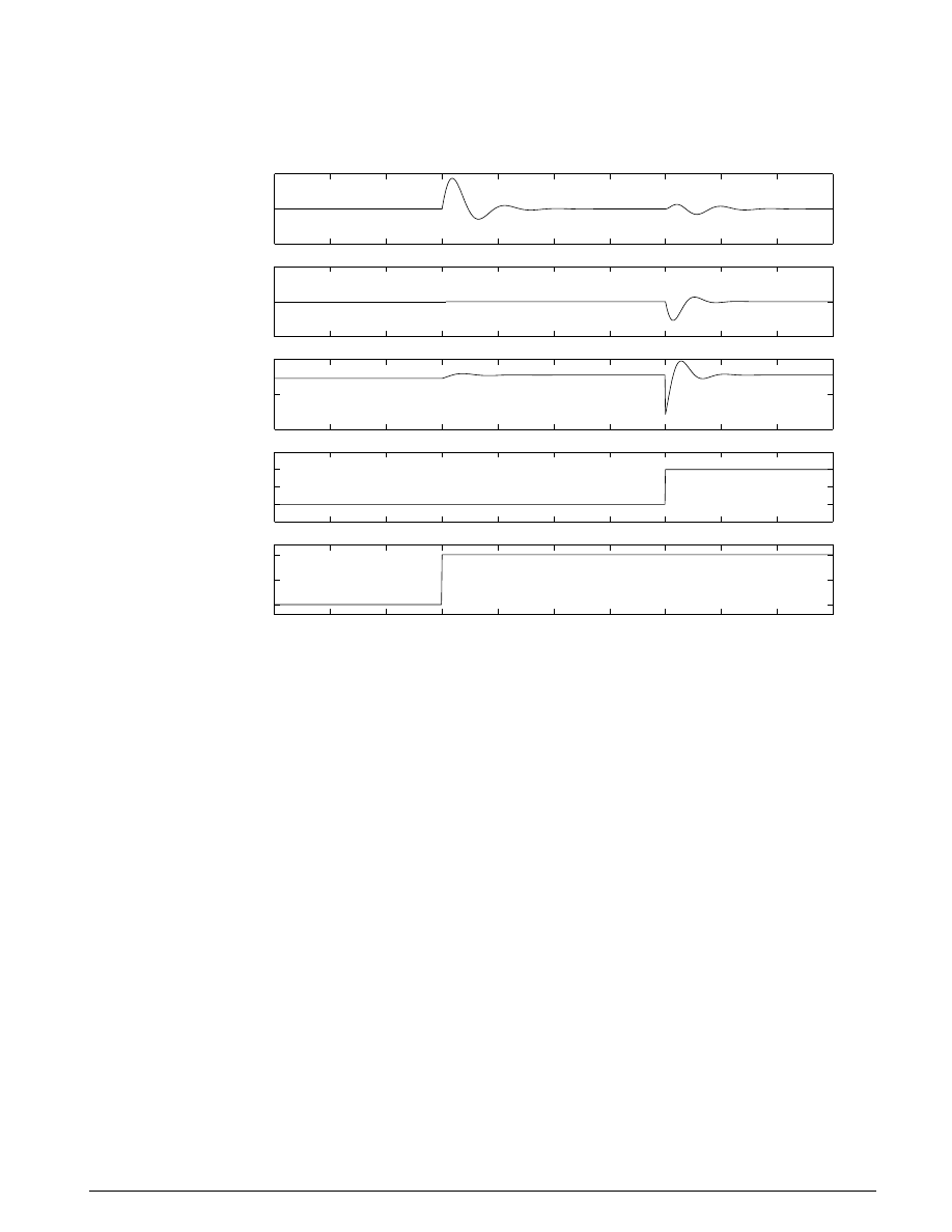
Results
B
ASELINE
M
ODEL
We simulated the model with the following data.
C
C
C
A
K
V
d
c
=
=
=
=
=
=
=
=
0.61
800 kg/m
2e- 8 m /sec/Pa
3e- 9 m /sec/Pa
7e8 Pa
0.001 m
5e4 N/m
2.5e- 5 m
3
3
3
3
3
ρ
β
1
2
30
We specified the pump flow as:
sec. m
3
/sec
[T, Q] =
0
0.005
0.04
0.005
0.04
0
0.05
0
0.05
0.005
0.1
0.005
The system thus initially steps to a pump flow of 0.005 m
3
/sec = 300 l/min, abruptly steps to zero at t =
0.04, then resumes its initial flow rate at t = 0.05.
The control valve starts with zero orifice area and ramps to 1e-4 m
2
during the 0.1 second simulation
time. With the valve closed, all of the pump flow goes to leakage so the initial pump pressure jumps to
p
10
=
Q/C
2
=
1667 KPa.
As the valve opens, pressures p
2
and p
3
build up while p
1
dips in response to the load increase as shown in
Figure 5.5. When the pump flow cuts off, the spring and piston act like an accumulator and p
3
, though
decreasing, is continuous. The flow reverses direction, so p
2
, though relatively close to
p
3
, falls abruptly.
At the pump itself, all of the backflow goes to leakage and
p
1
drops radically. This behavior reverses as the
flow is restored.
40
S
IMULINK
-S
TATEFLOW
T
ECHNICAL
E
XAMPLES
0
0.01
0.02
0.03
0.04
0.05
0.06
0.07
0.08
0.09
0.1
0
2
4
6
8
10
12
14
16
18
x 10
5
time (sec)
system pressures (Pa)
Baseline Hydraulic Pressure Response
p
1
p
2
p
3
p
1
p
2
p
3
p
1
p
2
p
3
Figure 5.5: Pressures in baseline simulation
The piston position is directly proportional to p
3
, where the hydraulic and spring forces balance as shown
in Figure 5.6. Discontinuities in the velocity at 0.04 and 0.05 seconds indicate negligible mass. The model
reaches a steady state when all of the pump flow again goes to leakage, now due to zero pressure drop
across the control valve. That is, p
3
= p
2
= p
1
= p
10
.
0
0.01
0.02
0.03
0.04
0.05
0.06
0.07
0.08
0.09
0.1
0
0.005
0.01
0.015
0.02
0.025
0.03
0.035
time (sec)
piston position (m)
Baseline Hydraulic Cylider
Figure 5.6: Baseline hydraulic cy linder p iston p osition

U
SING
S
IMULINK AND
S
TATEFLOW IN
A
UTOMOTIVE
A
PPLICATIONS
41
We have now tested the pump and actuator blocks and determined that they perform according to design.
We created a Simulink library and copied these blocks into it. After saving the library (
hydlib.mdl
), we
replaced the blocks in the original model with library copies. The model file,
hydcyl.mdl
, now contains
references to the library blocks rather than all of the details of the subsystems. This demonstrates how we
build master libraries of important system components. Other designers can now employ identical copies
of these blocks in other systems. Whenever improvements are made to the library blocks, Simulink
automatically incorporates the changes into each individual model.
Four Cylinder Model
We now construct a new model with a single pump and four actuators (Figure 5.7). The same pump
pressure p1 drives each cylinder assembly and the sum of their flows loads the pump. Although each of
the four control valves could be controlled independently, as in an active suspension system, in this case
all four receive the same commands, a linear ramp in orifice area from zero to 0.002 m
2
.
Four Cylinder Model
p1
A
p
x
qin
valve/cylinder/piston assembly 4
p1
A
p
x
qin
valve/cylinder/piston assembly 3
p1
A
p
x
qin
valve/cylinder/piston assembly 2
p1
A
p
x
qin
valve/cylinder/piston assembly 1
supply
pressure
p1
pump
Mux
positions
x1 (yellow)
x2 (purple)
x3 (blue)
x4 (red)
load
flow
control
valve
command
Double click for a model
with two hydraulic cylinders
interconnected by a rigid rod
Double click to run the
Simulation for 0.1 seconds
Figure 5.7: A single pump d riving four actuators
The pump flow begins at 0.005 m
3
/sec again for this system, then drops to half that value at t = 0.05 sec.
The parameters C
1
, C
2
, C
d
,
ρ
and V
30
are identical to the previous model. However, by assigning
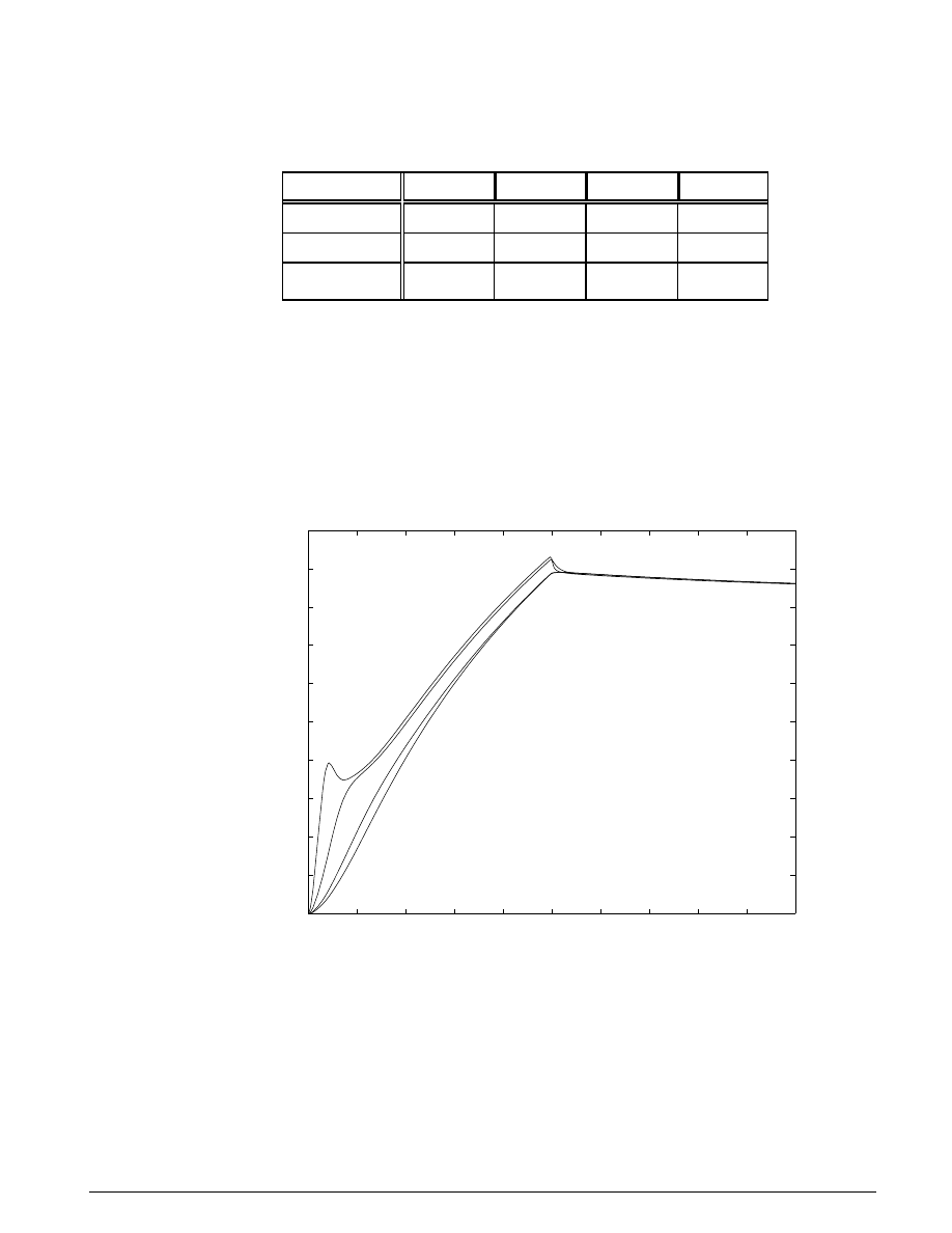
42
S
IMULINK
-S
TATEFLOW
T
ECHNICAL
E
XAMPLES
individual values for K, A
c
and, in one case,
β
, each of the four cylinders exhibit distinctive transient
responses. In relationship to the parameter values used above, the model characterizes the four actuators
according to Table 5.1.
Table 5.1: Parameter c omparison for individual actuators
The ratio of area/spring rate remains constant, so each case should have the same steady-state output.
The dominant time constant for each subsystem is proportional to A
c
2
/K, so we can expect case two to be
somewhat faster than the case one, and case three somewhat slower. In case four, the effective bulk
modulus of the fluid is significantly lower, as would be the case with entrained air. We thus expect this
softer case to respond more sluggishly than case one. The simulation results support these predictions.
0
0.01
0.02
0.03
0.04
0.05
0.06
0.07
0.08
0.09
0.1
0
0.002
0.004
0.006
0.008
0.01
0.012
0.014
0.016
0.018
0.02
time (sec)
piston position (m)
Piston Positions in Four Cylinder Example
x
1
x
2
x
3
x
4
Figure 5.8: Actuator Positions for Four-Cylinder Model
The initial jolt of flow at t = 0 responds like a pressure impulse, as seen by the four actuators (in Figure
5.8). The pump pressure p
1
, which is initially high, drops rapidly as all four loads combine to make a
high flow demand. During the initial transient (about four milliseconds), distinctive responses identify
the individual dynamic characteristics of each unit.
parameter
actuator 1
actuator 2
actuator 3
actuator 4
spring rate
K
K/4
4K
K
piston area
A
c
A
c
/4
4A
c
A
c
bulk modulus
β
β
β
β
/1000
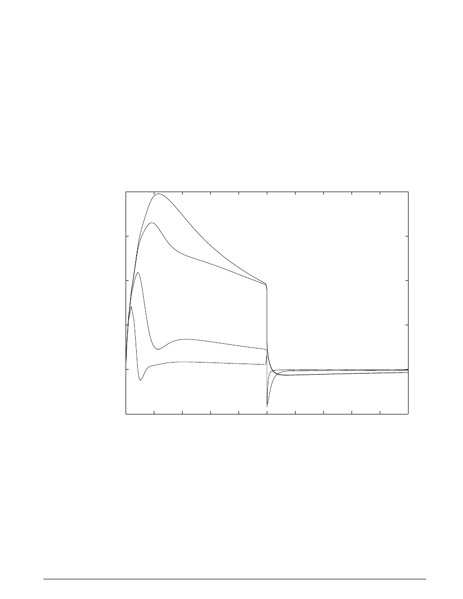
U
SING
S
IMULINK AND
S
TATEFLOW IN
A
UTOMOTIVE
A
PPLICATIONS
43
As predicted by the differences in parameter values, actuator two responds much faster than the baseline,
actuator one. The third and fourth devices are much slower because they require more oil to move the
same distance. In case three, the piston displaces more volume due to its larger cross-sectional area. In
case four, although the displaced volume is the same as in case one, the device requires more oil because it
is subsequently compressed.
The distinctions in behavior are blurred, however, as the pump pressure falls to the level within the
cylinders (in Figure 5.9). The individual responses blend into an overall system response which
maintains the flow balance between the components. At t = 0.05 seconds, the pump flow drops to a level
that is close to equilibrium and the actuator flows are nearly zero. The individual steady-state piston
positions are equal, as predicted by design.
0
0.01
0.02
0.03
0.04
0.05
0.06
0.07
0.08
0.09
0.1
-5
0
5
10
15
20
x 10
-4
time (sec)
actuator flow rate (m
3
/sec)
Flow Transients in Four Cylinder Example
q
1
q
2
q
3
q
4
Figure 5:9: Individual flow rates in four cylinder model
Two Cylinder Model with Load Constraints
In the final model (Figure 5.10), a rigid rod which supports a large mass interconnects two hydraulic
actuators. The model eliminates the springs as it applies the piston forces directly to the load. These forces
balance the gravitational force and result in both linear and rotational displacement.
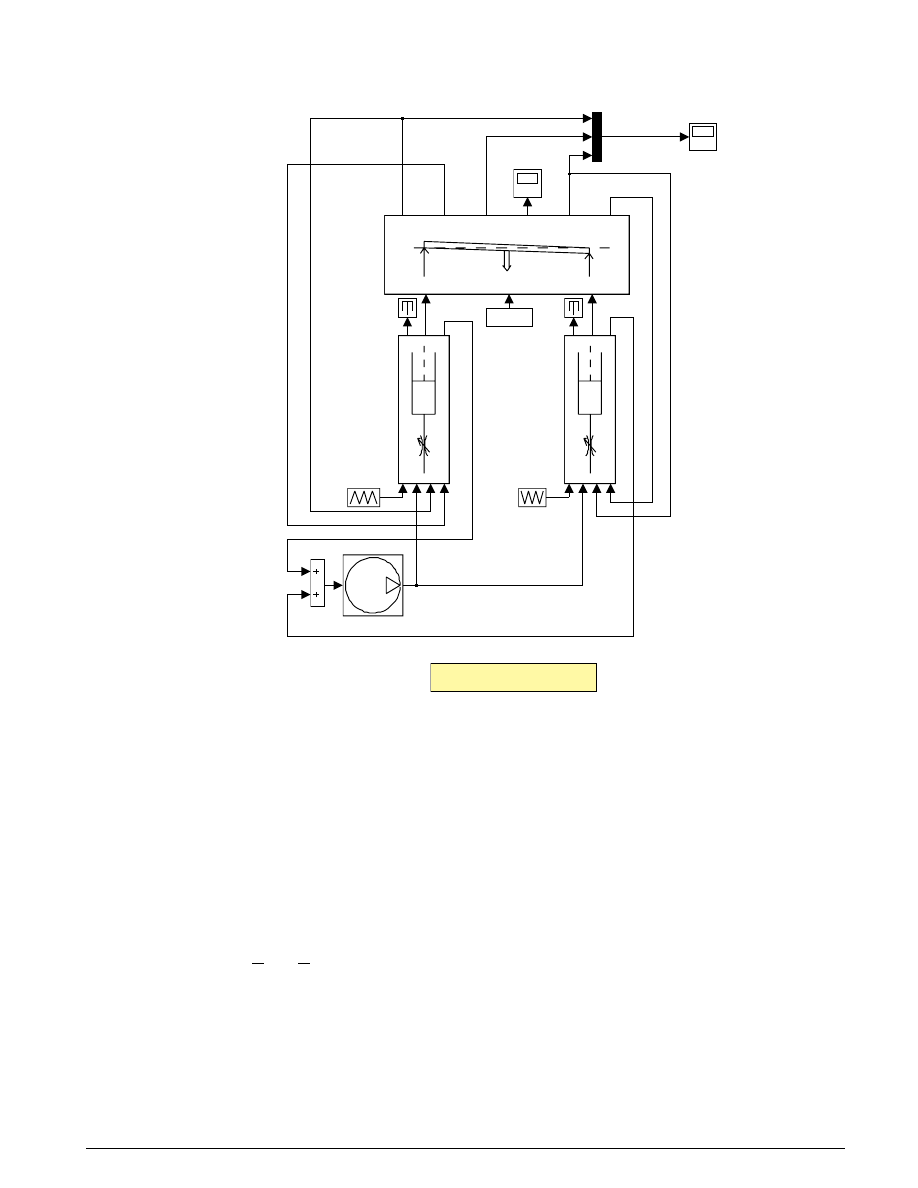
44
S
IMULINK
-S
TATEFLOW
T
ECHNICAL
E
XAMPLES
Two Cylinder Model with Connecting Rod
z (purple), za (blue)
& zb (yellow)
A
p1
x
xdot
p
F
qin
valve/cylider/piston
force assembly 2
A
p1
x
xdot
p
F
qin
valve/cylider/piston
force assembly 1
theta
(rad)
pump
Mux
orifice B
orifice A
load
flow
Double click to run the
Simulation for 0.1 seconds
Fb
Fext
Fa
zb
zbdot
z
theta
za
zadot
Mechanical
Load
- 9.81*M
supply pressure
Figure 5.10: Two hydraulic c ylinders with c onnecting rod
The load subsystem shown in Figure 5.11 solves the equations of motion, which we compute directly with
standard Simulink blocks. We assume the rotation angle is small.
Mz
F
F
F
z
M
F
F
F
I
L
F
L
F
I
L
b
a
ext
a
b
ext
b
a
˙˙
,
˙˙
=
+
+
=
=
=
=
=
−
=
=
=
displacement at center
total mass
piston forces
external force at center
angular displacement, clockwise
moment of inertia
rod length
θ
θ
2
2
Equation
5.6
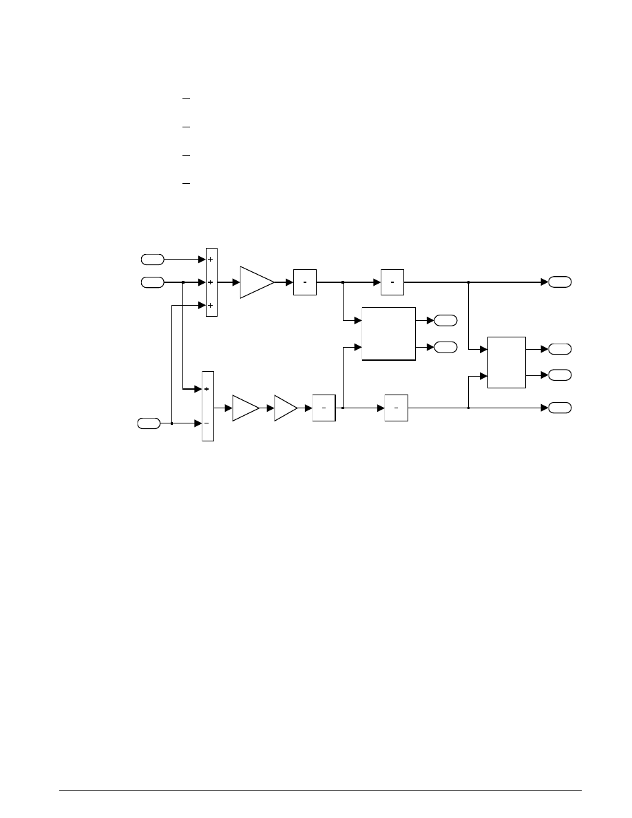
U
SING
S
IMULINK AND
S
TATEFLOW IN
A
UTOMOTIVE
A
PPLICATIONS
45
The positions and velocities of the individual pistons follow directly from the geometry.
z
z
L
z
z
L
z
z
L
z
z
L
z
z
a
b
a
b
a
b
= −
= +
= −
= +
=
2
2
2
2
θ
θ
θ
θ
˙
˙
˙
˙
˙
˙
,
piston displacements
Equation
5.7
Connecting Rod
6
zadot
2
zbdot
zdot
thetadot
zbdot
zadot
velocity
translation
z
theta
zb
za
position
translation
s
1
s
1
s
1
s
1
L/2
1/I
1/M
3
Fa
2
Fext
1
Fb
zdot
3
z
4
theta
1
zb
5
za
thetadot
Figure 5.11: Mechanical load subsystem
The parameters used in the simulation are identical to the first model, except:
L
Q
F
M
pump
ext
=
=
=
=
=
=
1.5m
M 2500 kg
I 100 kg- m
0.005 m /sec (constant)
C2 3e- 10 m /sec/Pa
-9.81 N
2
3
3
Although pump flow is constant in this case, the model controls the valves independently according to the
following schedule in Figure 5.12:
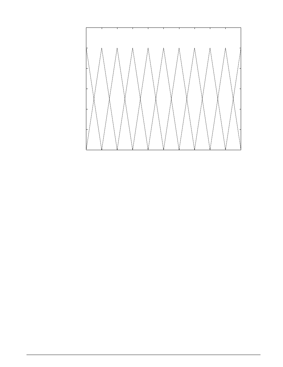
46
S
IMULINK
-S
TATEFLOW
T
ECHNICAL
E
XAMPLES
0
0.01
0.02
0.03
0.04
0.05
0.06
0.07
0.08
0.09
0.1
0
0.2
0.4
0.6
0.8
1
1.2
x 10
-5
System Control Valve Inputs
time (secs)
control valve orifice area (m
2
)
B
A
Figure 5.12: Complementary a ctuator c ontrol action
Figure 5.13 and Figure 5.14 show the simulation outputs of rod displacement and angle, respectively. The
response of z is typical of a type-one (integrating) system. The relative positions and the angular
movement of the rod illustrate the response of the individual actuators to their out-of-phase control
signals.
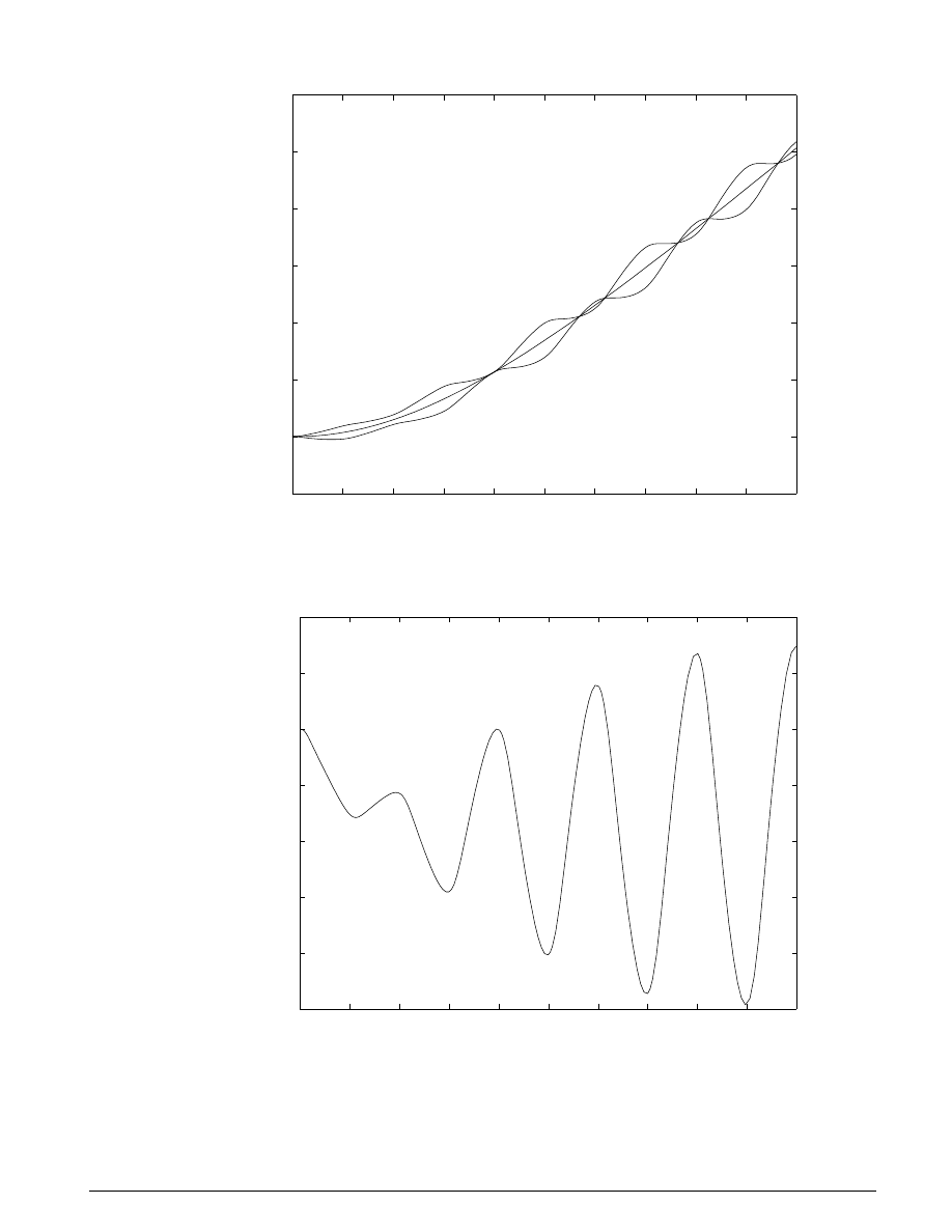
U
SING
S
IMULINK AND
S
TATEFLOW IN
A
UTOMOTIVE
A
PPLICATIONS
47
0
0.01
0.02
0.03
0.04
0.05
0.06
0.07
0.08
0.09
0.1
-2
0
2
4
6
8
10
12
x 10
-3
time (sec)
linear piston displacement (m)
Piston and Load Positions
z
a
z
z
b
Figure 5.13: Linear piston and load motion
0
0.01
0.02
0.03
0.04
0.05
0.06
0.07
0.08
0.09
0.1
-10
-8
-6
-4
-2
0
2
4
x 10
-4
time (sec)
load angular displacement (rad)
Two Cylinder Model Rotational Response
Figure 5.14: Rotational displacement of load

48
S
IMULINK
-S
TATEFLOW
T
ECHNICAL
E
XAMPLES
Conclusions
Simulink provides a productive environment for simulating hydraulic systems, offering enhancements
that provide enormous productivity in modeling and flexibility in numerical methods. The use of masked
subsystems and model libraries facilitates structured modeling with automatic component updates. That
is, as users modify library elements, the models that use the elements automatically incorporate the new
versions. Simulink can use differential-algebraic equations (DAEs) to model some fluid elements as
incompressible and others as compliant, allowing efficient solutions for complex systems of
interdependent circuits.
Models such as these will ultimately be used as part of overall plant or vehicle systems. The hierarchical
nature of Simulink allows independently developed hydraulic actuators to be placed, as appropriate, in
larger system models, for example, adding controls in the form of sensors or valves. In cases such as
these, tools from the M
ATLAB
Control System Toolbox can analyze and tune the overall closed-loop
system. The M
ATLAB
/Simulink environment can thus support the entire design, analysis, and modeling
cycle.

U
SING
S
IMULINK AND
S
TATEFLOW IN
A
UTOMOTIVE
A
PPLICATIONS
49
System Models in Simulink with Stateflow Enhancements

50
S
IMULINK
-S
TATEFLOW
T
ECHNICAL
E
XAMPLES
VI. F
AULT
-
T
OLERANT
F
UEL
C
ONTROL
S
YSTEM
Summary
The following example illustrates how to combine Stateflow with Simulink to efficiently model hybrid
systems. This type of modeling is particularly useful for systems that have numerous possible
operational modes based on discrete events. Traditional signal flow is handled in Simulink while
changes in control configuration are implemented in Stateflow.
The model described below represents a fuel control system for a gasoline engine. The system is highly
robust in that individual sensor failures are detected and the control system is dynamically reconfigured
for uninterrupted operation.
Analysis and
Similar to the engine model described earlier in this document, physical and empirical relationships
Physics
form the basis for the throttle and intake manifold dynamics of this model. The mass flow rate of air
pumped from the intake manifold, divided by the fuel rate which is injected at the valves, gives the air-fuel
ratio. The ideal, or stoichiometric mixture ratio provides a good compromise between power, fuel
economy, and emissions. A target ratio of 14.6 is assumed in this system.
Typically, a sensor determines the amount of residual oxygen present in the exhaust gas (EGO). This
gives a good indication of the mixture ratio and provides a feedback measurement for closed-loop control.
If the sensor indicates a high oxygen level, the control law increases the fuel rate. When the sensor detects
a fuel-rich mixture, corresponding to a very low level of residual oxygen, the controller decreases the fuel
rate.
Modeling
Figure 6.1 shows the top level of the Simulink model (
fuelsys.mdl
). The controller uses signals from
the system’s sensors to determine the fuel rate which gives a stoichiometric mixture. The fuel rate
combines with the actual air flow in the engine gas dynamics model to determine the resulting mixture
ratio as sensed at the exhaust.
The user can selectively disable each of the four sensors (throttle angle, speed, EGO and manifold absolute
pressure [MAP]), to simulate failures. Simulink accomplishes this with
Manual Switch
blocks. Double-
click on the block itself to change the position of the switch. Similarly, the user can induce the failure
condition of a high engine speed by toggling the switch on the far left. A
Repeating Table
block provides the
throttle angle input and periodically repeats the sequence of data specified in the mask.
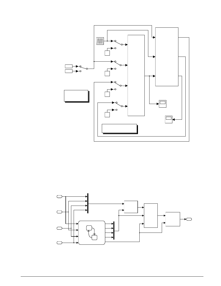
U
SING
S
IMULINK AND
S
TATEFLOW IN
A
UTOMOTIVE
A
PPLICATIONS
51
Use these switches to
simulate any combination
of sensor failures
Use this switch
to force the
engine to
overspeed
Fault Tolerant Fuel Control System
Choose Start from
the Simulation
menu to run
the model.
To toggle
a switch,
double click
on its icon.
throttle
sensor
throttle
command
speed
sensor
throttle
engine speed
EGO
MAP
fuel rate
fuel rate
controller
engine speed
throttle angle
fuel
o2_out
MAP
air/fuel ratio
engine
gas
dynamics
engine
speed
air/fuel
mixture ratio
300
Nominal
Speed
Metered Fuel
MAP
sensor
700
High
Speed
(rad./Sec.)
EGO
sensor
0
0
12
0
Figure 6.1: Simulink fuelsys model
The controller uses the sensor input and feedback signals to adjust the fuel rate to give a stoichiometric
ratio (Figure 6.2). The model uses four subsystems to implement this strategy: control logic, sensor
correction, airflow calculation, and fuel calculation. Under normal operation, the model estimates the
airflow rate and multiplies the estimate by the reciprocal of the desired ratio to give the fuel rate. Feedback
from the oxygen sensor provides a closed-loop adjustment of the rate estimation in order to maintain the
ideal mixture ratio.
fuel rate controller
1
fuel
rate
throt
speed
Ego
press
throtState
speedState
o2State
pressState
fuel_mode
control logic
Sensors
Failures
Corrected
Sensor correction and
Fault Redundancy
Mu
Mu
airflow
mode
fuel rate
Fuel Calculation
sens_in
Failures
mode
airflow
Airflow calculation
4
MAP
3
EGO
2
engine
speed
1
throtle
Figure 6.2: Fuel rate c ontroller subsystem
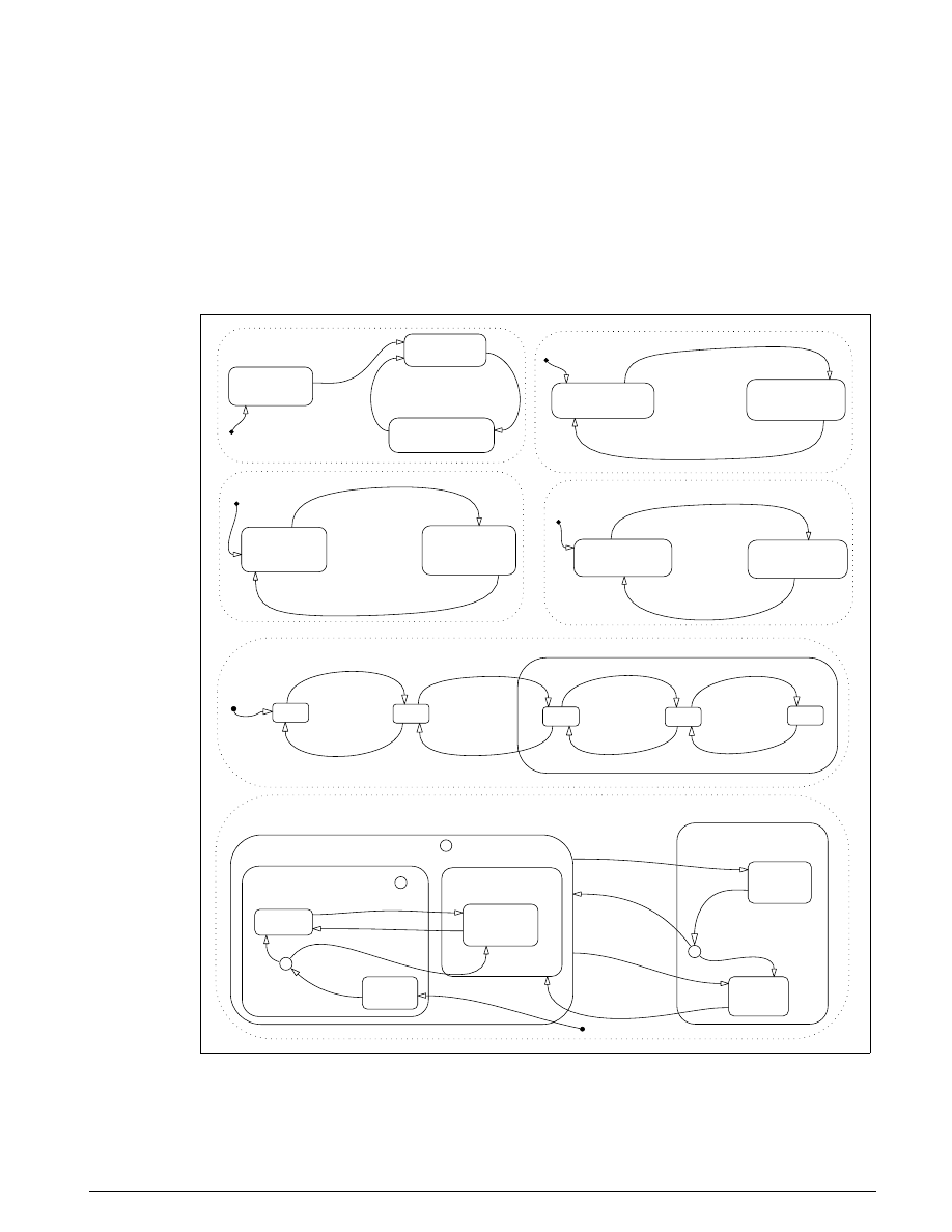
52
S
IMULINK
-S
TATEFLOW
T
ECHNICAL
E
XAMPLES
Control Logic
A single Stateflow chart, consisting of a set of six parallel states, implements the control logic in its
entirety. The four parallel states shown at the top of Figure 6.3 correspond to the four individual sensors.
The remaining two parallel states at the bottom consider the status of the four sensors simultaneously
and determine the overall system operating mode. The model synchronously calls the entire Stateflow
diagram at a regular sample time interval of 0.01 sec. This permits the conditions for transitions to the
correct mode to be tested on a timely basis.
Oxygen_Sensor_Mode
Pressure_Sensor_Mode
O2_normal
entry: o2State = 0
O2_warmup
entry: o2State = 1
press_fail
entry: pressState = 1
press_norm
entry: pressState = 0
O2_fail
entry: o2State = 1
Throttle_Sensor_Mode
Speed_Sensor_Mode
throt_fail
entry: throtState = 1
throt_norm
entry: throtState=0
speed_norm
entry: speedState = 0
speed_fail
entry: speedState = 1
Sens_Failure_Counter
MultiFail
FL0
FL1
FL4
FL2
FL3
Fueling_Mode
Fuel_Disabled
entry: fuel_mode = DISABLED
Running
Overspeed
Low_Emmisions
entry: fuel_mode = LOW
Rich_Mixture
entry: fuel_mode = RICH
Single_Failure
Normal
Shutdown
Warmup
H
H
[t > o2_t_thresh]
[press > max_press | press < min_press]
/Sens_Failure_Counter.INC
[Ego > max_ego]/
Sens_Failure_Counter.INC
[Ego < max_ego] /
Sens_Failure_Counter.DEC
[press > min_press & press < max_press] /
Sens_Failure_Counter.DEC
[throt> max_throt | throt < min_throt]/
Sens_Failure_Counter.INC
[speed==0 & press < zero_thresh]/
Sens_Failure_Counter.INC
[throt > min_throt & throt < max_throt]
/ Sens_Failure_Counter.DEC
[speed > 0] /
Sens_Failure_Counter.DEC
INC
INC
INC
INC
DEC
DEC
DEC
DEC
[ speed > max_speed ]
[in(speed_norm) & ...
speed < (max_speed - hys)]
[!in(MultiFail)]
[in(FL1)]
[in(FL0)]
[in(FL1)]
enter(MultiFail)
[in(MultiFail)]
[in(O2_normal)]
exit(MultiFail)
fuel rate
controller/control logic
Printed 14 Nov 1997 12:53:27
Figure 6.3: Control logic S tateflow diagram

U
SING
S
IMULINK AND
S
TATEFLOW IN
A
UTOMOTIVE
A
PPLICATIONS
53
When execution begins, all of the states start in their “normal” mode with the exception of the oxygen
sensor. The O2_warmup state is entered initially until time has exceeded the o2_t_thresh. The system
detects throttle and pressure sensor failures when their measured values fall outside their nominal
ranges. A manifold vacuum in the absence of a speed signal indicates a speed sensor failure. The oxygen
sensor also has a nominal range for failure conditions but, because zero is both the minimum signal
level and the bottom of the range, failure can be detected only when it exceeds the upper limit.
Regardless of which sensor fails, the model always generates the directed event broadcast
Sens_Failure_Counter.INC
. In this way the triggering of the universal sensor failure logic is
independent of the sensor. The model also uses a corresponding sensor recovery event,
Sens_Failure_Counter.DEC
. The
Sens_Failure_Counter
state keeps track of the number of failed
sensors. The counter increments on each
Sens_Failure_Counter.INC
event and decrements on each
Sens_Failure_Counter.DEC
event. The model uses a superstate,
MultiFail
,
to group all cases where
more than one sensor has failed.
The bottom parallel state represents the fueling mode of the engine. If a single sensor fails, operation
continues but the air/fuel mixture is richer to allow smoother running at the cost of higher emissions. If
more than one sensor has failed, the engine shuts down as a safety measure, since the air/fuel ratio
cannot be controlled reliably.
During the oxygen sensor warm-up, the model maintains the mixture at normal levels. If this is
unsatisfactory, the user can change the design by moving the warm-up state to within the
Rich_Mixture
superstate. If a sensor failure occurs during the warm-up period, the
Single_Failure
state is entered
after the warm-up time elapses. Otherwise, the
Normal
state
is activated at this time
.
We easily added a protective overspeed feature by creating a new state in the
Fuel_Disabled
superstate.
Through the use of history junctions, we assured that the chart returns to the appropriate state when the
model exits the overspeed state. As the safety requirements for the engine become better specified, we can
add additional shutdown states to the
Fuel_Disabled
superstate.
Sensor Correction
The Fault Correction block determines which sensors to use and which to estimate. Figure 6.4 shows the
block diagram for this subsystem. The failures input is a vector of logic signals that trigger the
application of estimates to each particular sensor. When a component of the signal is nonzero, it enables
the appropriate estimation subsystem and causes the switch relating to that signal to send the estimate as
the output. Since the estimation routines are within enabled subsystems, they do not introduce any
computational overhead when they are not needed.
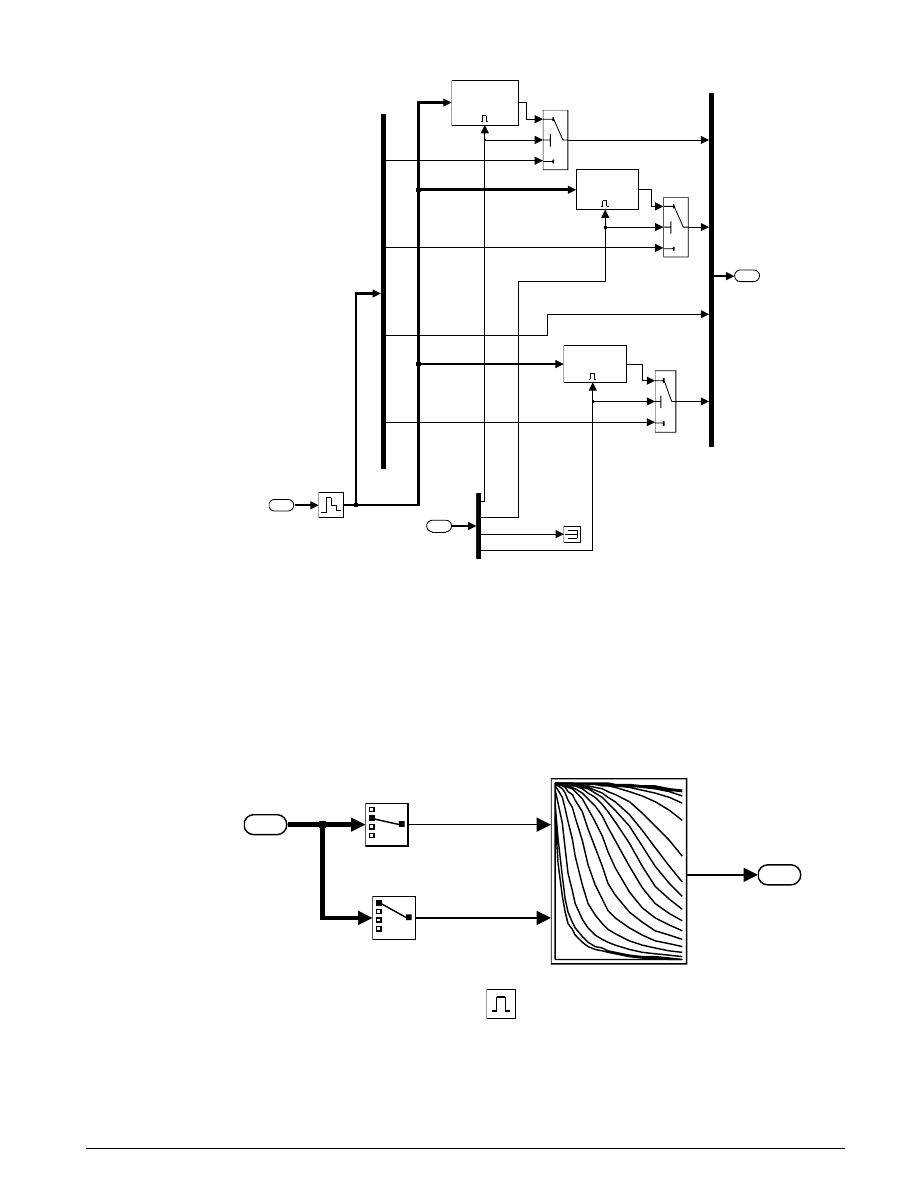
54
S
IMULINK
-S
TATEFLOW
T
ECHNICAL
E
XAMPLES
Sensors
throtle
Throttle Estimate
Sensors
we
Speed Estimate
Sensors
map
MAP Estimate
m
m
2
1
Sensors
Failures
throttle
EGO
speed
MAP
throttle
sensor
failure
speed sensor failure
1
Corrected
pressure sensor failure
6.4: Sensor c orrection and fault redundancy
The sensors input to the Correction block is the vector of raw sensor values. When there are no faults, the
input simply passes on as the output signal. When a fault exists, the appropriate estimation block uses
this signal to recover the missing component. Figure 6.5 shows an estimation example of the algorithm
for the manifold pressure sensor.
MAP Estimation
1
map
Pressure Estimate (2D)
Enable
1
Sensors
speed
throttle
Figure 6.5: Manifold a bsolute p ressure reconstruction
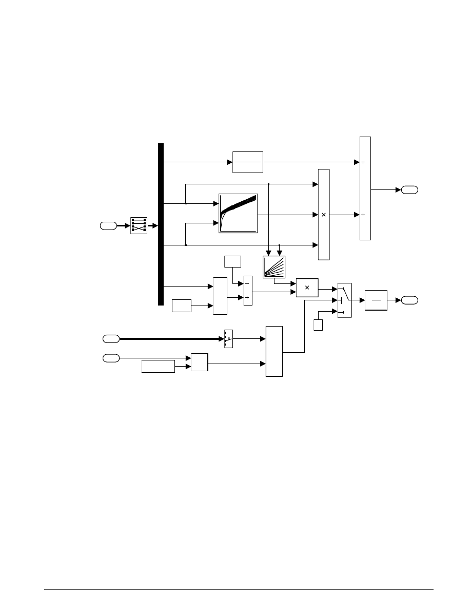
U
SING
S
IMULINK AND
S
TATEFLOW IN
A
UTOMOTIVE
A
PPLICATIONS
55
Airflow Calculation
The
Airflow Calculation
block (Figure 6.6) is the location for the central control laws. The block estimates
the intake air flow to determine the fuel rate which gives the appropriate air/fuel ratio. Closed-loop
control adjusts the estimation according to the residual oxygen feedback in order to maintain the mixture
ratio precisely. Even when a sensor failure mandates open-loop operation, the most recent closed-loop
adjustment is retained to best meet the control objectives.
Intake Airflow Estimation and Closed Loop Correction
Feedback Control
Feedforward Control
hold
integrator
LOW
0.01z-0.01
z - 0.8
Throttle transient
correction
<=
~=
Ramp
Rate (Ki)
Pumping Constant
0.5
Oxygen Sensor
Switching Threshold
NOR
T
z -1
Integrator
em
0
0.5
3
mode
2
Failures
1
sens_in
e2
manifold pressure, Pm
engine speed, N
throttle angle
O2 fail
(warmup)
not normal operation
EGO, residual
exhaust oxygen
e1
enable integration
e0
2
feedback
correction
1
est.
air
flow
Figure 6.6: Airflow Estimation and Correction
The engine’s intake air flow can be formulated as the product of the engine speed, the manifold pressure
and a time-varying scale factor.

56
S
IMULINK
-S
TATEFLOW
T
ECHNICAL
E
XAMPLES
q
N
V
P
RT
C
N P
NP
N
V
P
R
T
cd
m
pump
m
m
cd
m
=
=
=
=
=
=
=
=
=
4
π
η
η
(
,
)
,
intake mass flow
engine speed (rad/sec)
engine cylinder displacement volume
volumetric efficiency
manifold pressure
specific gas constant
gas temperature
Equation 6.1
C
pump
is computed by a lookup table and multiplied by the speed and pressure to form the initial flow
estimate. During transients, the throttle rate, with the derivative approximated by a high-pass filter,
corrects the air flow for filling dynamics. The control algorithm provides additional correction according
to Eqs. 6.2:
e
e
K
N P
e
e
e
i
m
0
1
0
2
1
0 5
0 5
0 5
0 5
0
=
≤
−
>
=
=
. ,
.
. ,
.
(
,
)
˙
,
,
EGO
EGO
LOW mode with valid EGO signal
RICH, DISABLE or EGO warmup
Equation 6.2
The nonlinear oxygen sensor, modeled with a hyperbolic tangent in the engine gas Mixing and
Combustion subsystem, provides a meaningful signal when in the vicinity of 0.5 volt. The raw error in
the feedback loop is thus detected with a switching threshold, as indicated in Equation 6.2. If the value is
low (the mixture is lean), the original air estimate is too small and needs to be increased. Conversely,
when the oxygen sensor output is high, the air estimate is too large and needs to be decreased. Integral
control is utilized so that the correction term achieves a level that brings about zero steady-state error in
the mixture ratio.
The normal closed-loop operation mode, LOW, adjusts the integrator dynamically to minimize the error.
The integration is performed in discrete time, with updates every 10 milliseconds. When operating open-
loop however, in the RICH or O2 failure modes, the feedback error is ignored and the integrator is held.
This gives the best correction based on the most recent valid feedback.
Fuel Calculation
The Fuel Calculation subsystem (Figure 6.7) sets the injector signal to match the given airflow
calculation and fault status. The first input is the computed airflow estimation. This is multiplied with
the target fuel/air ratio to get the commanded fuel rate. Normally the target is stoichiometric, 1/14.6.
e
2
=
closed–loop correction
e
0
, e
1
, e
2
=
intermediate error signals
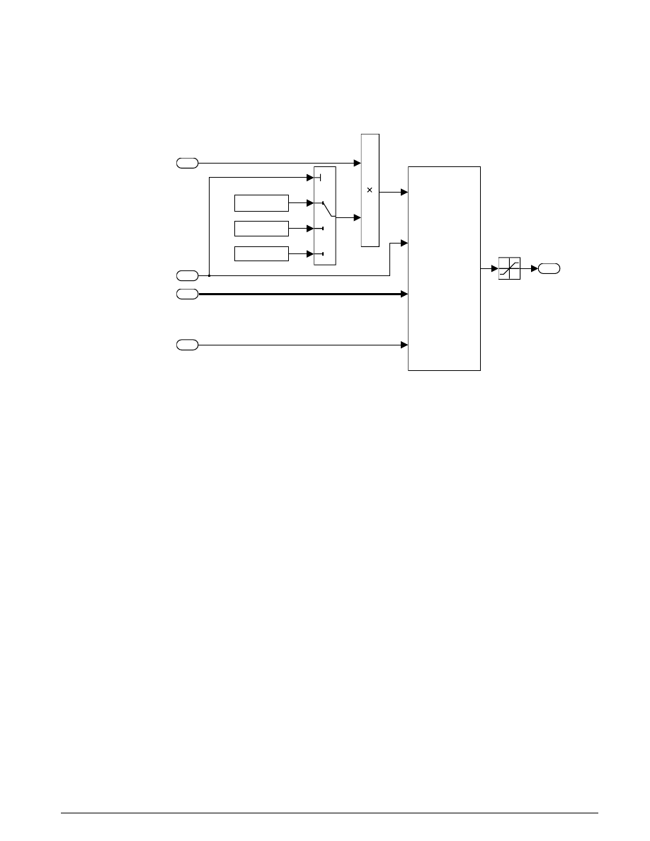
U
SING
S
IMULINK AND
S
TATEFLOW IN
A
UTOMOTIVE
A
PPLICATIONS
57
When a sensor fault occurs, the Stateflow control logic sets the mode input to a value of 2 or 3 (RICH or
DISABLED) so that the mixture is either slightly rich of stoichiometric or is shut down completely.
Fuel Rate Calculation
1
fuel
rate
limit
output
feedforward fuel rate
mode
Failures
feedback correction
fuel rate
Switchable
Compensation
0
Shutdown
1/(14.6*0.8)
F/A Rich
1/14.6
F/A Norm
4
mode
3
Failures
2
correction
1
est.
air
flow
Figure 6.7: Fuel Calculation Subsystem
The Fuel Calculation subsystem (Figure 6.7) employs adjustable compensation (Figure 6.8) in order to
achieve different purposes in different modes. In normal operation, phase lead compensation of the
feedback correction signal adds to the closed-loop stability margin. In RICH mode and during EGO
sensor failure (open loop), however, the composite fuel signal is low-pass filtered to attenuate noise
introduced in the estimation process. The end result is a signal representing the fuel flow rate which, in
an actual system, would be translated to injector pulse times.
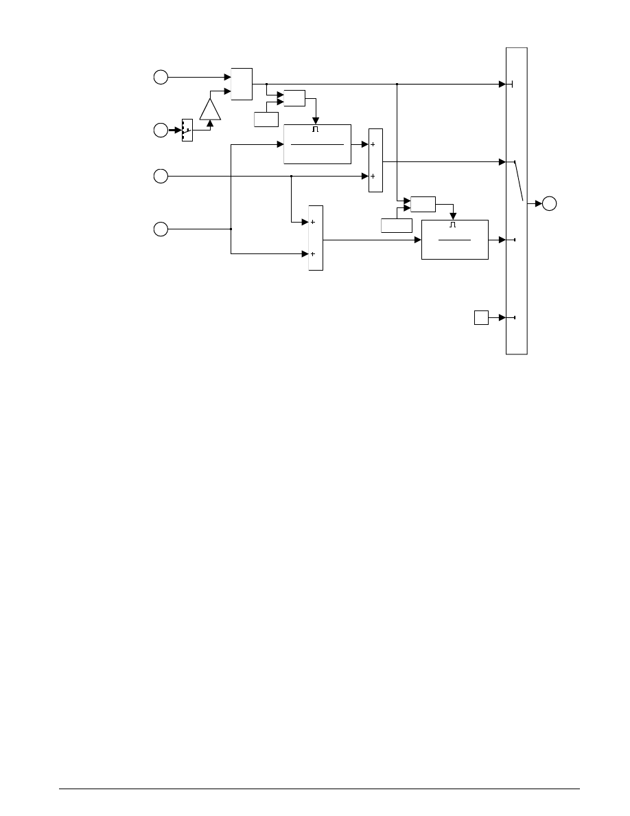
58
S
IMULINK
-S
TATEFLOW
T
ECHNICAL
E
XAMPLES
Loop Compensation and Filtering
2
0
Shutoff
Mode
==
==
0.25918
z - 0.74082
RICH Mode
O2 fail
(warmup)
max
8.7696z - 8.5104
z - 0.74082
LOW Mode
RICH
LOW
4
feedback
correction
3
Failures
2
mode
1
feedforward
fuel rate
1
Fuel Rate
Figure 6.8: Switchable c ompensation
Results and
Simulation results are shown in Figure 6.9 and Figure 6.10. The simulation is run with a throttle input
Conclusions
that ramps from 10 to 20 degrees over a period of two seconds, then back to 10 degrees over the next two
seconds. This cycle repeats continuously while the engine is held at a constant speed so that the user can
experiment with different fault conditions and failure modes. To simulate a sensor failure, double-click
on its associated switch (see Figure 6.1). Repeat this operation to toggle the switch back for normal
operation.
Figure 6.9 compares the fuel flow rate under fault-free conditions (baseline) with the rate applied in the
presence of a single failure in each sensor individually. Note, in each case, the nonlinear relationship
between fuel flow and the triangular throttle command (shown qualitatively on its Simulink icon). In
the baseline case, the fuel rate is regulated tightly, exhibiting a small ripple due to the switching nature of
the EGO sensor’s input circuitry. In the other four cases the system operates open loop. The control
strategy is proven effective in maintaining the correct fuel profile in the single-failure mode. In each of
the fault conditions, the fuel rate is essentially 125% of the baseline flow, fulfilling the design objective of
80% rich.
Figure 6.10 plots the corresponding air/fuel ratio for each case. The baseline plot shows the effects of
closed-loop operation. The mixture ratio is regulated very tightly to the stoichiometric objective of 14.6.
The rich mixture ratio is shown in the bottom four plots of Figure 6.10. Although they are not tightly
regulated, as in the closed-loop case, they approximate the objective of air/fuel = 0.8(14.6) = 11.7.
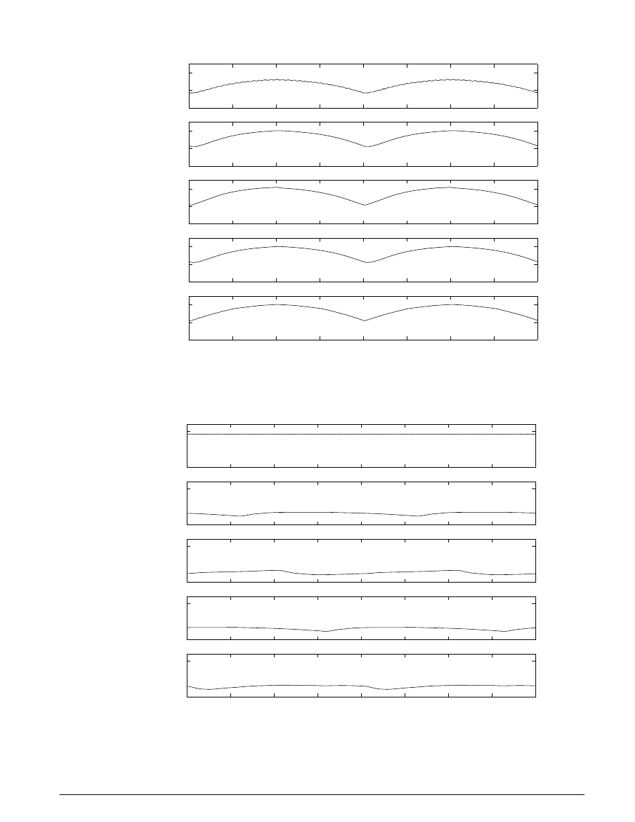
U
SING
S
IMULINK AND
S
TATEFLOW IN
A
UTOMOTIVE
A
PPLICATIONS
59
0
1
2
FaultTolerant Fuel Control System: Fuel Rate
g/sec
baseline
0
1
2
g/sec
throttle sensor failed
0
1
2
g/sec
speed sensor failed
0
1
2
g/sec
EGO sensor failed
0
1
2
3
4
5
6
7
8
0
1
2
g/sec
time (sec)
MAP sensor failed
Figure 6.9: Comparative results for simulated fuel rate
10
15
FaultTolerant Fuel Control System: Air/Fuel Ratio
baseline
10
15
throttle sensor failed
10
15
speed sensor failed
10
15
EGO sensor failed
0
1
2
3
4
5
6
7
8
10
15
time (sec)
MAP sensor failed
Figure 6.10: Comparative results for simulated a ir/fuel ratio
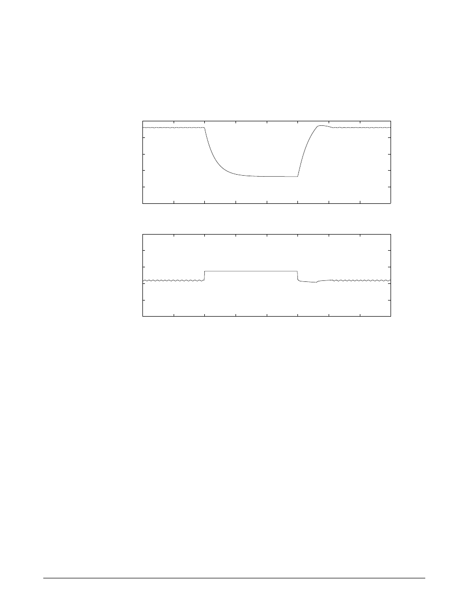
60
S
IMULINK
-S
TATEFLOW
T
ECHNICAL
E
XAMPLES
The transient behavior of the system is shown in Figure 6.11. With a constant 12
°
throttle angle and the
system in steady-state, a throttle failure is introduced at t = 2 and corrected at t = 5. At the onset of the
failure, the fuel rate increases immediately. The effects are seen at the exhaust as the rich ratio propagates
through the system. The steady-state condition is then quickly recovered when closed-loop operation is
restored.
10
11
12
13
14
15
air/fuel ratio
Response to Throttle Failure
0
1
2
3
4
5
6
7
8
0
0.5
1
1.5
2
2.5
fuel rate (g/sec)
time (sec)
Figure 6.11: Transient response to fault d etection
During simulation, this behavior can also be observed from the Stateflow perspective. By enabling
animation in the Stateflow debugger, the state transitions are highlighted in Figure 6.3 as the various
states are activated. The sequence of activation is indicated by changing colors. This closely coupled
synergy between Stateflow and Simulink fosters the modeling and development of complete control
systems. An engineer’s concepts can develop in a natural and structured fashion with immediate visual
feedback reinforcing each step.
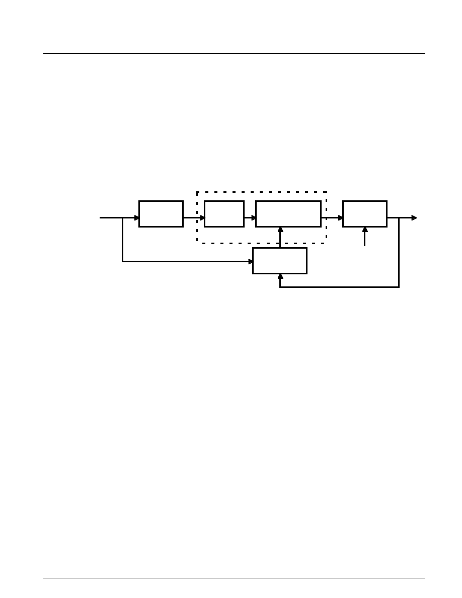
U
SING
S
IMULINK AND
S
TATEFLOW IN
A
UTOMOTIVE
A
PPLICATIONS
61
VII.
A
UTOMATIC
T
RANSMISSION
C
ONTROL
Summary
In this example, Simulink is used to model an automotive drivetrain. Stateflow enhances the Simulink
model with its representation of the transmission control logic. Simulink provides a powerful
environment for the modeling and simulation of dynamic systems and processes. In many systems,
though, supervisory functions like changing modes or invoking new gain schedules must respond to
events that may occur and conditions that develop over time. As a result, the environment requires a
language capable of managing these multiple modes and developing conditions. In the following
example, Stateflow demonstrates its strength in this capacity by performing the function of gear selection
in an automatic transmission. This function is combined with the drivetrain dynamics in a natural and
intuitive manner by incorporating a
Stateflow
block in the Simulink block diagram.
Figure 7.1: Drivetrain system block diagram
Figure 7.1 shows the power flow in a typical automotive drivetrain. Nonlinear ordinary differential
equations model the engine, four-speed automatic transmission, and vehicle. The model directly
implements these as modular Simulink subsystems. On the other hand, the logic and decisions made in
the transmission controller (TCU) do not lend themselves to well-formulated differential or difference
equations; these are better suited to a Stateflow representation. Stateflow monitors the events which
correspond to important relationships within the system and takes the appropriate action as they occur.
Analysis and
The engine receives input in the form of the throttle opening, as commanded by the driver. It is connected
Physics
to the impeller of the torque converter which couples it to the transmission
.
I N
T
T
N
I
T
f (
N )
T
ei
e
e
i
e
ei
e
e
i
˙
=
−
=
=
=
=
engine speed
engine + impeller moment of inertia
throttle,
= engine torque
impeller torque
1
Equation
7.1
The input-output characteristics of the torque converter can be expressed as functions of the engine speed
and the turbine speed. In this example, the direction of power flow is always assumed to be from impeller
to turbine.
Engine
Torque
Converter
Gearset and
Shift Mechanism
Vehicle
Dynamics
Transmission
Control Unit
Throttle
brake
T r a n s m i s s i o n
mph

62
S
IMULINK
-S
TATEFLOW
T
ECHNICAL
E
XAMPLES
T
N
K
K
f N
N
i
e
in
e
=
=
(
/
)
(
/
)
2
2
N
T
R T
R
f N
N
in
t
TQ i
TQ
in
e
=
=
=
=
=
=
turbine (torque converter output) speed
transmission input speed
turbine torque
torque ratio
3
(
/
)
The transmission model is expressed as static gear ratios, assuming small shift times.
R
f gear
T
R T
N
R
N
T T
N
N
R
TR
out
TR in
in
TR
out
in
out
in
out
TR
=
=
=
=
=
=
4
(
)
,
,
transmission input and output torque
transmission input and output speed
transmission ratio
Equation
7.3
The final drive, inertia, and a dynamically varying load constitute the vehicle dynamics.
I N
R
T
T
I
N
R
T
f N
v
w
fd
out
load
v
w
fd
load
w
˙
(
)
(
)
=
−
=
=
=
=
=
vehicle inertia
wheel speed
final drive ratio
load torque
5
Equation
7.4
The load torque includes both the road load and brake torque. The road load is the sum of frictional and
aerodynamic losses.
T
mph
R
R
mph
T
T
R
R
T
mph
load
load
load
brake
load
load
load
brake
=
+
+
=
=
=
=
sgn(
)(
)
,
0
2
2
0
2
load torque
friction and aerodynamic drag coefficients
brake torque
vehicle linear velocity
Equation. 7.5
The model programs the shift points for the transmission according to a schedule, such as is shown in
Figure 7.2. For a given throttle in a given gear, there is a unique vehicle speed at which an upshift takes
place; the simulation operates similarly for a downshift.
=
capacity or K–factor
Equation 7.2
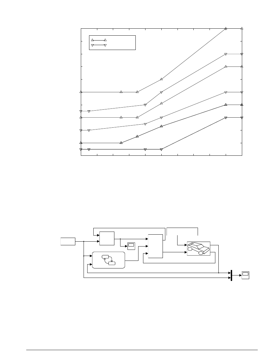
U
SING
S
IMULINK AND
S
TATEFLOW IN
A
UTOMOTIVE
A
PPLICATIONS
63
0
10
20
30
40
50
60
70
80
90
100
0
10
20
30
40
50
60
70
80
90
100
1-2
2-3
3-4
2-1
3-2
4-3
throttle (%)
vehicle speed (mph)
transmission shift points
upshift
downshift
Figure 7.2: Shift Schedule
Modeling
The Simulink model (
sf_car.mdl
) is composed of modules which represent the engine, transmission
and vehicle, with an additional shift logic block to control the transmission ratio. User inputs to the
model are in the form of throttle (%) and brake torque (ft-lb). The diagram in Figure 7.3 shows the
overall model.
Choose Start from
the Simulation menu
to run the simulation.
sf_car.mdl
vehicle mph
(yellow)
& throttle %
Ne
gear
Nout
Ti
Tout
transmission
9 40;15 100;10
throttle
schedule
throttle
vehicle_speed
gear
shift_logic
engine RPM
[0 0;100 0;101 400;200 400]
brake
schedule
Vehicle
Mu
Ti
throttle
Ne
Engine
impeller torque
output torque
transmission speed
vehicle
speed
Figure 7.3: Overall simulation model
The Engine subsystem consists of a two-dimensional table that interpolates engine torque vs. throttle and
engine speed. In accordance with Equation 7.1, the model subtracts the impeller torque, divides the
difference by the inertia and then numerically integrates the quotient to compute the engine speed.
Figure 7.4 shows the composite engine subsystem.
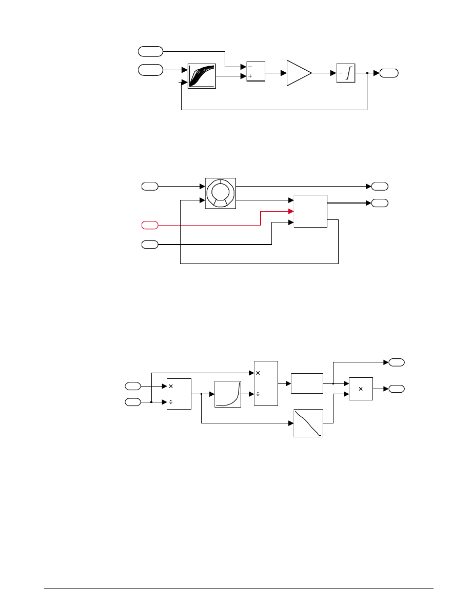
64
S
IMULINK
-S
TATEFLOW
T
ECHNICAL
E
XAMPLES
1
Ne
s
1
speed
1/Iei
engine + impeller
inertia
engine
torque
2
throttle
1
Ti
Figure 7.4: Engine subsystem
The torque converter and the block which implements the various gear ratios make up the transmission
subsystem, as shown in Figure 7.5.
2
Tout
1
Ti
Tin
gear
Nout
Tout
Nin
transmission
ratio
Torque
Converter
3
Nout
2
gear
1
Ne
output torque
impeller torque
transmission output speed
engine speed
turbine speed
turbine torque
Figure 7.5: Transmission subsystem
The torque converter is a masked subsystem, under which the model computes the relationships of
Equation 7.2. The parameters entered into the subsystem are a vector of speed ratios (N
in
/N
e
) and vectors
of K-factor (f
2
) and torque ratio (f
3
) corresponding to the speed ratio data. Figure 7.6 shows the subsystem
implementation.
TORQUE CONVERTER
2
Tt
1
Ti
turbine
speed
ratio
quotient
u^2
impeller
Torque
ratio
K
factor
2
Nin
1
Ne
Figure 7.6: Torque c onverter subsystem
The transmission ratio block determines the ratio R
TR
(gear), shown in Table 7.1 and computes the
transmission output torque and input speed, as indicated in Equation 7.3. The ratios used progress from
low to another underdrive ratio, one-to-one and overdrive.
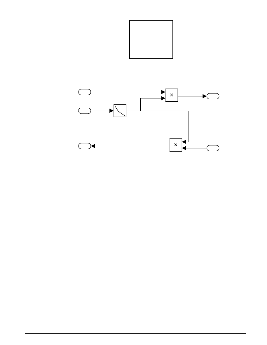
U
SING
S
IMULINK AND
S
TATEFLOW IN
A
UTOMOTIVE
A
PPLICATIONS
65
gear
R
TR
1
2 393
2
1 450
3
1 000
4
0 677
.
.
.
.
Table 7.1: Transmission Gear Ratios
Figure 7.7 shows the block diagram for the subsystem that realizes this ratio in torque and speed.
2
Nin
1
Tout
Product1
Product
LookUp
Table
3
Nout
2
gear
1
Tin
Figure 7.7: Transmission gear ratio subsystem
The Stateflow block labeled
shift_logic
implements gear selection for the transmission. The Stateflow
Explorer is utilized to define the inputs as throttle and vehicle speed and the output as the desired gear
number. Two dashed
AND
states keep track of the gear state and the state of the gear selection process. The
overall chart is executed as a discrete-time system, sampled every 40 mSec. The Stateflow diagram shown
in Figure 7.8 illustrates the functionality of the block.
The shift logic behavior, explained in the following, can be observed during simulation by enabling
animation in the Stateflow debugger. The
selection_state
, which is always active, begins by
performing the computations indicated in its
during
function. The model computes the upshift and
downshift speed thresholds as a function of the instantaneous values of gear and throttle (see Figure 7.2).
While in
steady_state
, the model compares these values to the present vehicle speed to determine if a
shift is required. If so, it enters one of the
confirm
states
(
upshift_confirm
or
downshift_confirm
)
,
which records the time of entry.
If the vehicle speed no longer satisfies the shift condition, while in the
confirm
state, the model ignores the
shift and it transitions back to
steady_state
. This prevents extraneous shifts due to noise conditions. If
the shift condition remains valid for a duration of
Tconfirm
, the model transitions through the lower
junction and, depending on the current gear, it broadcasts one of the shift events. Subsequently, the model
again activates
steady_state
after a transition through one of the central junctions. The shift event,
which is broadcast to the
gear_selection
state, activates a transition to the appropriate new gear.
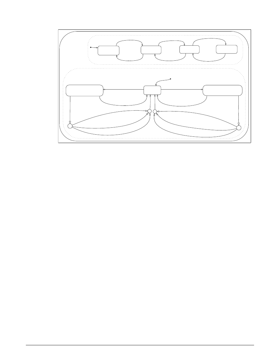
66
S
IMULINK
-S
TATEFLOW
T
ECHNICAL
E
XAMPLES
gear_selection/
gear_state
fourth/
entry: gear = 4;
third/
entry: gear = 3;
second/
entry: gear = 2;
first/
entry: gear = 1;
selection_state/
during: down_threshold = ml(’interp2([1:4],downth, downtab, %g, %g)’, gear, throttle);...
up_threshold = ml(’interp2([1:4],upth, uptab, %g, %g)’, gear, throttle);
downshift_confirm/
entry: tdn = t;
upshift_confirm/
entry: tup = t;
steady_state
UPSHIFT34
UPSHIFT12
UPSHIFT23
DOWNSHIFT43
DOWNSHIFT32
DOWNSHIFT21
[vehicle_speed < down_threshold]
[vehicle_speed > up_threshold]
[vehicle_speed > down_threshold]
[vehicle_speed < up_threshold]
[t-tup >= Tconfirm & ...
vehicle_speed >= up_threshold]
[t-tdn >= Tconfirm & ...
vehicle_speed <= down_threshold]
[gear ==4]/DOWNSHIFT43
[gear == 3]/UPSHIFT34
[gear == 3]/DOWNSHIFT32
[gear == 2]/UPSHIFT23
[gear == 2]/DOWNSHIFT21
[gear == 1]/UPSHIFT12
shift_logic
Printed 11Sep1997 16:52:48
Figure 7.8: Stateflow diagram of the transmission shift logic
For example, if the vehicle is moving along in second gear with 25% throttle, the state
second
is active
within
gear_state
, and
steady_state
is active in the
selection_state
. The
during
function of the latter
finds that an upshift should take place when the vehicle exceeds 30 mph. At the moment this becomes
true, the model enters the
upshift_confirm
state and sets the local variable
tup
to the current time by its
entry action. While in this state, if the vehicle speed remains above 30 mph until the elapsed time (
t -
tup
) reaches
Tconfirm
(0.1 Sec), the model satisfies the transition condition leading down to the lower
right junction. This also satisfies the condition [
gear
== 2
] on the transition leading from here to
steady
_
state
, so the model now takes the overall transition from
upshift_confirm
to
steady_state
and broadcasts the event
UPSHIFT23
as a transition action. Consequently, the transition from second to
third is taken in
gear_state
which completes the shift logic.
The vehicle dynamics (Figure 7.9) use the net torque to compute the acceleration and integrate it to
compute the vehicle speed, per Equation 7.4 and Equation 7.5. In this example, we again use a masked
subsystem for the vehicle submodel. The parameters entered in the mask menu are the final drive ratio,
the polynomial coefficients for drag friction and aerodynamic drag, the wheel radius, vehicle inertia, and
initial transmission output speed.
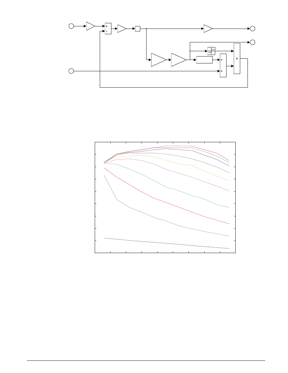
U
SING
S
IMULINK AND
S
TATEFLOW IN
A
UTOMOTIVE
A
PPLICATIONS
67
2
transmission
output speed
1
vehicle
speed
1/s
wheel
speed
1/Iv
vehicle
inertia
signed
load
f(u)
road load
60/5280
mph
2*pi*Rw
linear speed
Rfd
final drive
ratio
Rfd
final
drive
ratio
2
transmission
output torque
1
brake torque
Figure 7.9: Vehicle dynamics subsystem
Results
The engine torque map, torque converter characteristics, and road load data used in the simulations are
shown in the three plots which follow (Figure 7.10, Figure 7.11, and Figure 7.12).
500
1000
1500
2000
2500
3000
3500
4000
4500
5000
-100
-50
0
50
100
150
200
250
300
350
engine speed (RPM)
engine torque (ft-lb)
Engine Torque Map f
1
0% throttle
20% throttle
30%
40%
50%
60%
70%
100%
Figure 7.10: Engine map
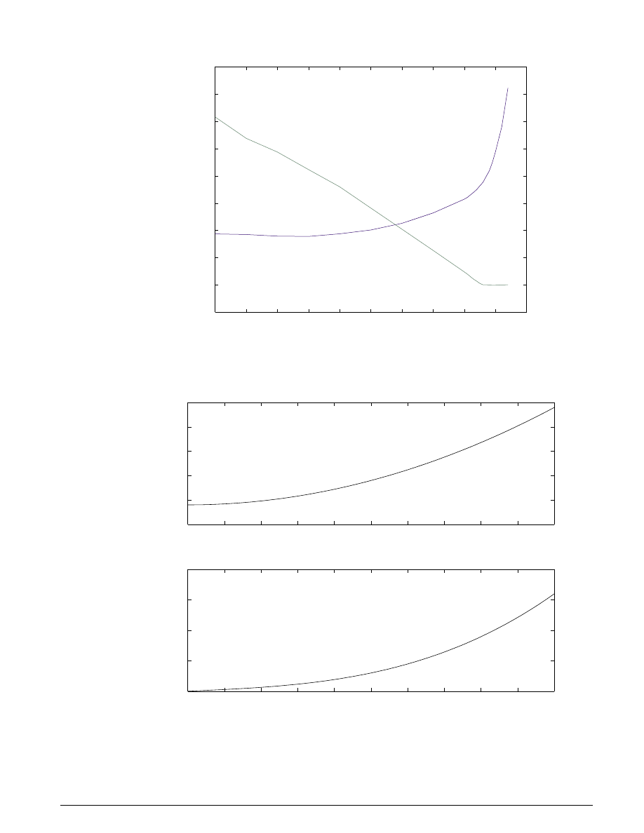
68
S
IMULINK
-S
TATEFLOW
T
ECHNICAL
E
XAMPLES
0
0.1
0.2
0.3
0.4
0.5
0.6
0.7
0.8
0.9
1
80
100
120
140
160
180
200
220
240
260
speed ratio, N
in
/N
e
K-f
actor (RPM/sqr
t(ft-lb))
Torque Converter Characteristics, f
2
, f
3
1.0
2.0
Torque Ratio
K-factor
Figure 7.11: Torque c onverter c haracteristics
0
50
100
150
200
250
torque (ftlb)
Vehicle Road Load, f
5
0
10
20
30
40
50
60
70
80
90
100
0
20
40
60
80
vehicle speed (mph)
power (HP)
Figure 7.12: Vehicle road load or d rag torque
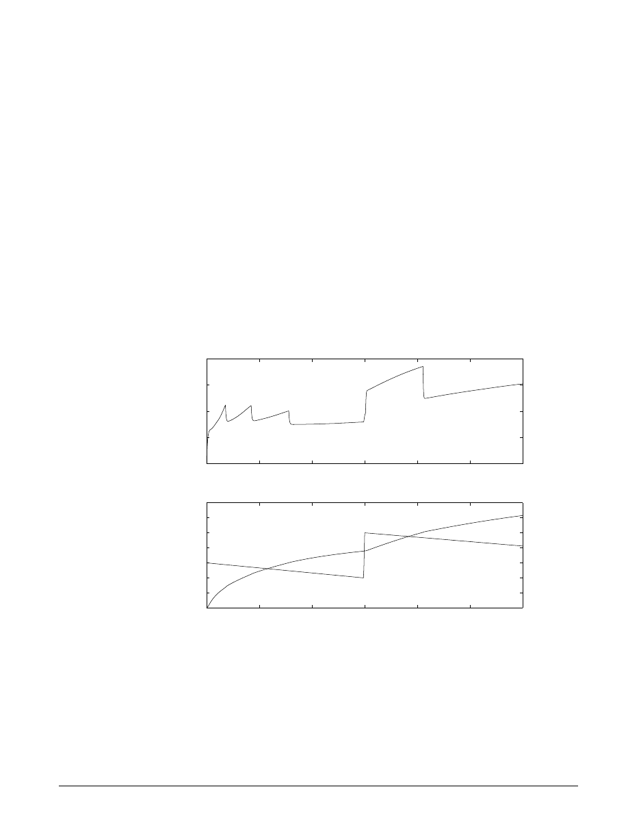
U
SING
S
IMULINK AND
S
TATEFLOW IN
A
UTOMOTIVE
A
PPLICATIONS
69
The first simulation uses the following throttle schedule:
throttle
=
0
60
14 9
40
15
100
100
0
200
0
.
The first column corresponds to time; the second column corresponds to throttle opening in percent. In
this case we do not apply the brake (0 ft-lb). The vehicle speed starts at zero and the engine at 1000 RPM.
Figure 7.13 shows the plot for the baseline results, using the default parameters. As the driver steps to
60% throttle at t = 0, the engine immediately responds by more than doubling its speed. This brings
about a low speed ratio across the torque converter and, hence, a large torque ratio (see Figs. 7.6 and 7.11).
The vehicle accelerates quickly (no tire slip is modeled) and both the engine and the vehicle gain speed
until about t = 2, at which time a 1-2 upshift occurs. The engine speed characteristically drops abruptly,
then resumes its acceleration. The 2-3 and 3-4 upshifts take place at about four and eight seconds,
respectively. Notice that the vehicle speed remains much smoother due to its large inertia.
1000
2000
3000
4000
5000
Baseline Automatic Transmission Simulation
engine speed (RPM)
0
5
10
15
20
25
30
0
20
40
60
80
100
120
140
time (sec)
vehicle speed (mph) & throttle (%)
throttle %
vehicle mph
Figure 7.13: Initial simulation time history
At t = 15, the driver steps the throttle to 100% as might be typical of a passing maneuver. The
transmission downshifts to third gear and the engine jumps from about 2600 to about 3700 RPM. The
engine torque thus increases somewhat, as well as the mechanical advantage of the transmission. With
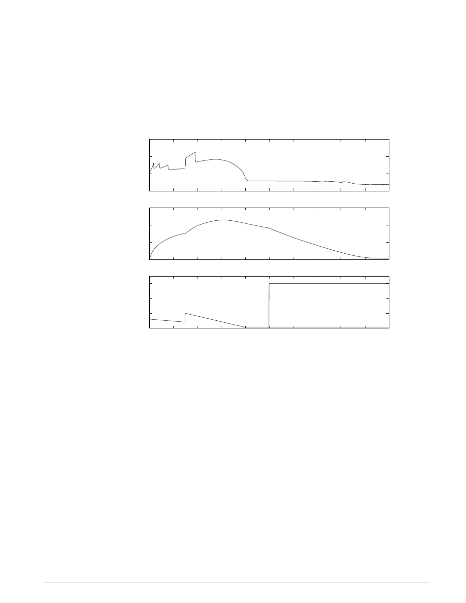
70
S
IMULINK
-S
TATEFLOW
T
ECHNICAL
E
XAMPLES
continued heavy throttle, the vehicle accelerates to about 100 mph and then shifts into overdrive at about t
= 21. The vehicle cruises along in fourth gear for the remainder of the simulation.
Figure 7.14 shows the results of a second simulation. The behavior for the first fifteen seconds is the same
as above, but the throttle subsequently drops to about 5% at 40 seconds. This is followed by a step in brake
torque at t = 50. Again, the large vehicle inertia dominates the dynamics as it eventually slows down to a
crawl. The engine speed downshifts occur at about 72, 80 and 90 seconds, ending in first gear.
0
50
100
150
vehicle speed (mph)
0
2000
4000
6000
engine speed (RPM)
Acceleration and Braking Maneuvers
0
10
20
30
40
50
60
70
80
90
100
0
100
200
300
time (sec)
throttle (%) & torque (ftlb)
throttle
brake
Figure 7.14: Vehicle simulation with a cceleration and b raking
Conclusions
We can easily enhance this basic system in a modular manner, for example, by replacing the engine or
transmission with a more complex model. We can thus build up large systems within this structure via
step-wise refinement. The seamless integration of Stateflow control logic with Simulink signal
processing enables the construction of a model which is both efficient and visually intuitive.
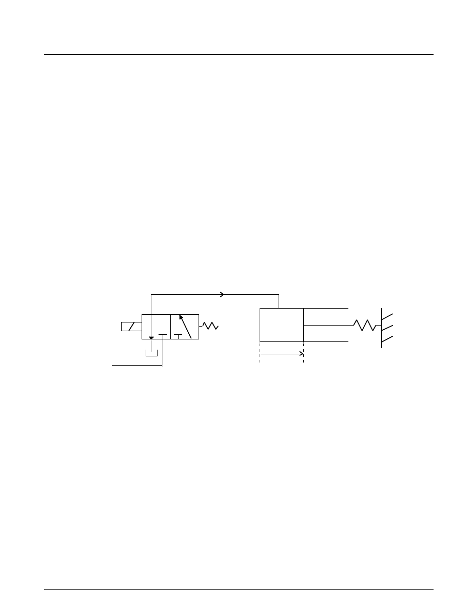
U
SING
S
IMULINK AND
S
TATEFLOW IN
A
UTOMOTIVE
A
PPLICATIONS
71
VIII. E
LECTROHYDRAULIC
S
ERVO
C
ONTROL
Summary
In this example we develop a Simulink model for a hydraulic servomechanism controlled by a pulse-
width modulated (PWM) solenoid. This might represent a motion control system in an industrial or
manufacturing setting, or a subsystem that controls the position of a valve in an automotive or aerospace
application. Nonlinear differential equations are used to model the magnetic, hydraulic and mechanical
components; discrete-time difference equations represent the controller. A behavioral model in Stateflow
implements the electronic circuit which generates the PWM waveforms and regulates the solenoid
current. Although a detailed power electronic model could be developed in Simulink, the Stateflow
description provides the required functionality and speeds development.
Figure 8.1 shows a hydraulic schematic for the mechanism. The objective of the system is to position the
load x
p
so that it follows commands issued in the form of a time-varying set point r
set
. An electronic
controller compares these commands to feedback measurements of x
p
and generates a PWM control
signal at a rate of 50 Hz. The PWM duty cycle is the percentage of the 20 millisecond period for which the
valve directly supplies oil to the control pressure developed in the cylinder behind the piston, p
c
. For the
remainder of the period, the valve vents p
c
to exhaust. The composite flow q
net
thus controls p
c
which
develops an actuating force against the piston. This forces the spring-loaded piston to its position x
p
such
that it follows the reference trajectory r
set
.
Figure 8.1: Solenoid v alve and h ydraulic actuator
We chose PWM control to regulate the net valve flow with its on/off duty ratio rather than relying on the
strict mechanical tolerances of a continuous valve. This sequentially turns the solenoid completely on or
off , rather than attempting to control it to a precise intermediate position. The tradeoff is that a
disturbance is introduced into the system at the PWM frequency. As a result, we must take care that this
is adequately attenuated by the low-pass response of the mechanical system. We can evaluate this
requirement by constructing a simulation at the design phase rather than waiting for experimental parts.
Analysi s and
PWM S
OLENOID
Physics
The model of the solenoid-controlled PWM valve includes three parts:
Magnetic circuit
Armature motion
Valve flows
p
c
A
p
P
s
K
sp
q
net
x
p
PWM
Solenoid
Valve
Cylinder and Piston
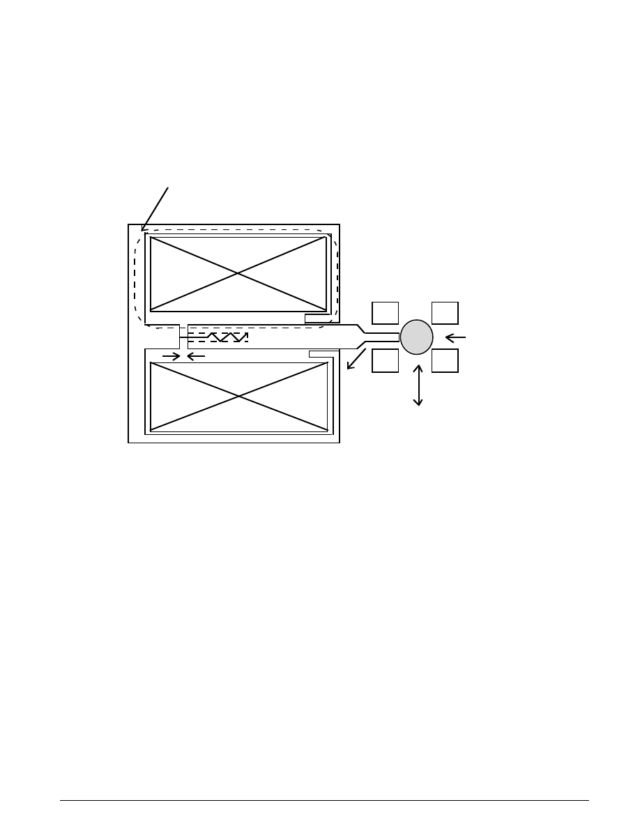
72
S
IMULINK
-S
TATEFLOW
T
ECHNICAL
E
XAMPLES
Figure 8.2 shows a cross-sectional view of a typical solenoid valve of this type. The enclosure, armature
and pole piece are steel, and the coil is wound around the armature/pole axis. With no current, the
internal spring forces the armature and ball to the right against the hydraulic force. This blocks the
supply pressure P
s
and opens a path from control pressure to exhaust. When the solenoid is energized, the
armature and pole come together and the pressure force shuttles the ball to open the supply port and block
the exhaust port.
Figure 8.2: Pulse-Width Modulated Solenoid Valve
Consider first the magnetic circuit. Faraday’s law determines the flux. We assume that fringing and
leakage flux are negligible, as are eddy currents.
˙
(
)/
,
φ
φ
=
−
=
=
=
=
=
v
iR
N
v
i
R
N
sol
sol
flux
solenoid voltage
current
winding resistance
number of turns
The magnetomotive force required to develop this flux is broken up into components for the steel and the
air gap. Although the majority of the circuit’s reluctance is concentrated at the air gap, the nonlinear
properties of the steel components, such as saturation and hysteresis, can limit performance.
P
s
armature
coil
p
c
exh
pole
air gap
flux path
control
pressure
supply
pre ssure

U
SING
S
IMULINK AND
S
TATEFLOW IN
A
UTOMOTIVE
A
PPLICATIONS
73
MMF
MMF
MMF
MMF
H
g
MMF
H
L
MMF
H
L
air
steel
air
air
steel
steel steel
steel
=
+
=
=
=
=
=
magnetomotive force
magnetic field intensity
g = length of air gap
magnetic circuit length in steel
Equation 8.1
Within the steel, the flux density, B, is a nonlinear function of H, dependent upon the material properties.
We also assume that the area, A, which relates
φ
and B at the air gap, applies uniformly for the steel path.
B
A
f(H
)
H
A
steel
air
=
=
=
=
=
=
φ
µ
µ
/
flux density
cross- sectional area at air gap
permeability of air
0
0
The solenoid force,
F
sol
, and current that result are:
F
B A
i
MMF N
sol
=
=
0 5
2
0
.
/
/
µ
The armature responds to the solenoid force, as well as the hydraulic and spring forces.
mx
F
A P
K x
C x
x
g
g
m
A
P
K
C
sol
o s
s
v
o
s
s
v
˙˙
˙
max
=
+
−
−
=
=
−
=
=
=
=
=
armature position
mass
supply orifice area
supply pressure
return spring rate
damping rate
Equation 8.2
The net oil flow directed from the valve to the actuator,
q
net
, is the supply flow less the exhaust flow.
q
q
q
q
K A
P
p
P
p
x
x
q
K A
p
x
balltravel
x
balltravel
p
K
net
s
ex
s
o
o
s
c
s
c
ex
o
o
c
c
o
=
−
=
−
−
>
=
=
<
=
=
=
sgn(
)
,
,
,
,
control pressure
flow coefficient
0
0
0
0
Equation 8.3

74
S
IMULINK
-S
TATEFLOW
T
ECHNICAL
E
XAMPLES
Actuator Dynamics
The actuator assembly moves the piston against a spring as a function of the control pressure developed
behind it. Assuming negligible leakage,
˙
˙
,
p
V
q
x A
V
x A
x
A
c
net
p
p
p
p
p
p
=
−
(
)
=
=
=
=
=
β
β
fluid bulk modulus
fluid volume
piston position
actuator (piston) area
Equation 8.4
The actuator’s equation of motion, dominated by the relatively large hydraulic and spring forces, is
simply:
M x
p A
K x
M
K
p p
c
p
sp p
p
sp
˙˙
,
=
−
=
=
net actuator mass
spring rate
Equation 8.5
Electronic Controls
We employ a discrete-time PI (proportional + integral) control law to
1. Achieve zero steady-state error to step changes in the position set point, and
2. Compensate for the low-frequency actuator dynamics to improve response speed.
dutycycle
K
K
z
r
x
p
I
set
p
=
+
−
−
1
(
)
Equation 8.6
The integral term is essential because the null duty cycle, or equilibrium control input, is subject to
uncertainty and will change with the system’s operating point. The proportional part contributes phase
lead at low frequency which is essential for stability.
Equation 8.6 computes the PWM duty cycle as a function of position error. The duty cycle is applied to a
50 Hz pulse train and the power electronics convert the pulse signal to solenoid current. Digital and
analog integrated circuits are available to perform these functions, so we use a behavioral model, rather
than a highly detailed physical model. The behavior is best described in terms of the circuit’s reaction to
the commands it receives and the response of its load. Figure 8.3 shows an idealized example.
At the beginning of each 20 millisecond period, the PWM pulse turns on and must pull the solenoid
armature up against the pole piece to open the valve to supply pressure. Hence, the driver circuit applies
the full supply voltage to achieve the fastest initial rise in current. The solenoid maintains this condition
until the current has risen to the level at which the magnetic and hydraulic forces overcome the spring
and move the armature.
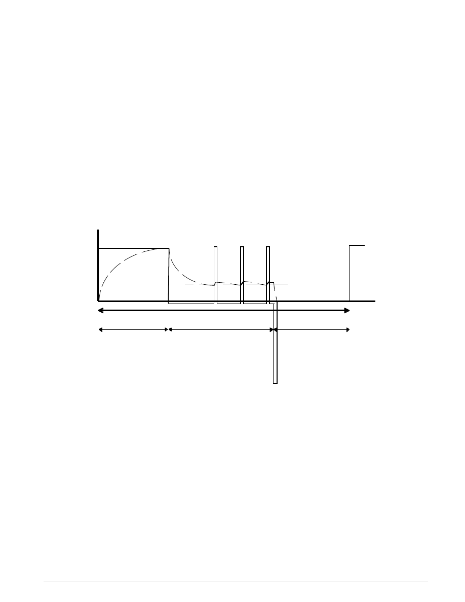
U
SING
S
IMULINK AND
S
TATEFLOW IN
A
UTOMOTIVE
A
PPLICATIONS
75
Once the armature has been pulled in, the air gap is very small and somewhat less current is needed to
hold the armature in place. The driver thus regulates the current at a lower level for the remainder of the
“on” portion of the cycle. Typically, a switch-mode regulator controls the “hold” current. This technique
alternatively applies the supply voltage to the solenoid and then allows the field to collapse slowly
(shunted by a freewheel diode). This is significantly more efficient, in terms of power, than linear
regulation.
At the end of each pulse, the armature releases so that the ball returns to its original position and the
valve opens to exhaust. We achieve this by opening the solenoid circuit so that the magnetic field
collapses quickly. Typically, we employ a zener diode to limit the large negative EMF while still allowing
a fast decay. The current then remains at zero for the duration of the “off” time until the next cycle
begins.
In this way, we divide the “on” portion of each pulse into two phases: “pull-in” and “hold.” The “off”
portion is characterized by the initial rapid decay, followed by zero voltage and current. The diagram in
Figure 8.3 illustrates this scenario.
Figure 8.3: Current c ontrol within pulses
Modeling
Figure 8.4 shows the top-level system block diagram (
sf_electrohydraulic.mdl
). The set point block
consists of a signal generator and a step function which are added to give wide flexibility to the user in
specifying the set point. The controller is a straightforward discrete-time subsystem. We implemented the
PWM driver circuit in Stateflow, but it functions just like the other subsystems at the block diagram level.
We refined the solenoid valve into three parts, as described above. The actuator model, consisting of the
cylinder pressurization and piston motion subsystems, completes the overall system model.
V
s
I
pull
I
hold
v o l tag e
current
20 mSec
pull in
hold
off
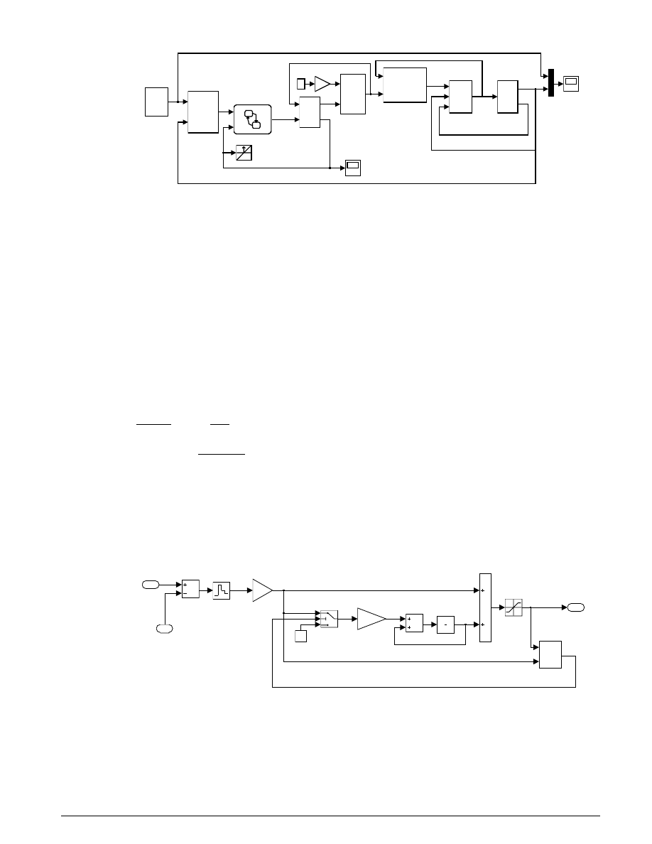
76
S
IMULINK
-S
TATEFLOW
T
ECHNICAL
E
XAMPLES
electrohydraulic servomechanism
control pressure
armature position
net flow
valve flows
solenoid
current (A)
set point
(yellow)
and
piston position
set point
position
command
pc
xp
xpdot
piston motion
qnet
xp
xpdot
pc
cylinder
pressurization
Fball
Fsol
stroke
armature
motion
Ps
Supply
Pressure
duty_cycle
i
v
PWM_driver_ckt
Mux
x
vsol
Fsol
isol
Magnetic
Circuit
Ao
set point
feedback
duty cycle
Controller
rset
solenoid
voltage
piston
position
control
pressure
Figure 8.4: Servo model using Simulink and Stateflow
Controller
The controller samples the position error and generates a new solenoid duty cycle every 20 milliseconds.
The duty cycle consists of a component that is proportional to the error plus a component that is
proportional to the integral of the error. The model realizes the integration in the z domain with feedback
around a 1/z block that places a pole at z = 1. The integral gain, as labeled in the diagram, (Figure 8.5) is
fixed with respect to the proportional gain. An overall loop gain, K
a
, adjusts both while keeping their
ratio, hence the transfer function zero, constant. While in the linear operating range:
duty cycle
error
K
K
z
K
z
K
z
a
I
a
I
=
+
−
=
− −
−
1
1
1
1
(
)
Equation 8.7
The model limits the computed duty cycle so that it never falls below the minimum time to open the
valve, nor exceeds the time at which the valve remains continuously open. Whenever it reaches either of
these limits, the integrator holds constant (zero input) until the error is of the appropriate sign to pull it
away from the limit.
proportional + integral control
controller
1
duty cycle
sampled
error
dc
e1
nothold
prevent
windup
Ka
loop
gain
0.1332
integral
gain
z
1
Saturation
0
2
feedback
1
set point
Figure 8.5: Discrete-time c ontroller subsystem
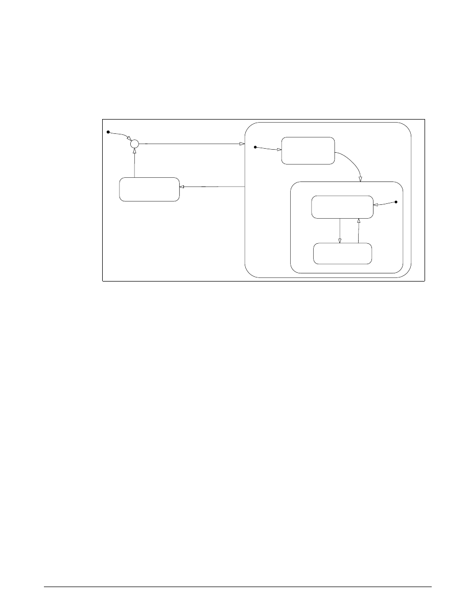
U
SING
S
IMULINK AND
S
TATEFLOW IN
A
UTOMOTIVE
A
PPLICATIONS
77
PWM Driver Circuit
The solenoid driver circuit uses the computed duty cycle to generate the PWM waveform. The solenoid
voltage is applied in order to achieve the desired current, force, and hence, valve flow. We modeled this
with a Stateflow block, which uses duty cycle and solenoid current as inputs and computes voltage as an
output. Figure 8.6 shows the Stateflow diagram for the model.
energize_solenoid
pull_in_current/
entry : v = Vs;
solenoid_off/
entry : v = -(i > 0)*Vz;
during: v = -(i > 0)*Vz;
regulate_hold_current
freewheel/
entry: v = -(i > 0)*Vd;
during: v = -(i > 0)*Vd;
hold/
entry : v = Vs;
/ton = 0;
/toff = ton + duty_cycle*Tpwm/100;
[t >= ton]
[i >= Ipull]
[t > toff]/ton += Tpwm;
[ i <= Ihold-deltai]
[i >= Ihold + deltai]
PWM_driver_ckt
Printed 12Sep1997 12:59:58
Figure 8.6: Stateflow diagram for the PWM d river c ircuit
Each PWM cycle begins with the local variable ton equal to the current simulation time. The
unconditional transition which begins the cycle computes toff, the time at which the “on” portion of the
pulse ends.
toff = ton + duty_cycle*Tpwm/100;
Equation 8.8
Tpwm
is a M
ATLAB
workspace variable representing the pulse period. The system enters the
energize
_
solenoid
state and, by default, the
pull
_
in
_
current
state. As described above, the driver
circuit connects the supply voltage to the output for this phase of the pulse. Once the current reaches
Ipull
, the worst-case current required to pull in the armature, it enters the
regulate_hold_current
state. A diode in the freewheel state shunts the coil which clamps the solenoid voltage at -Vd. When the
current falls to the hold level, the system alternates between the hold and freewheel states to regulate it to
Ihold
±
deltai
.
When the time reaches t = toff, it exits the
energize_solenoid
state, regardless of which of the
pull
-in,
freewheel
or
hold
states is currently active. This is achieved by drawing the transition directly from the
superstate boundary to the
solenoid_off
state. The value of
ton
, the beginning of the next cycle, is updated
at this time. While in the
solenoid_off
state, the coil connects to the zener voltage, -Vz, until the field
collapses and the current falls to zero, as described in the
entry
and
during
actions.
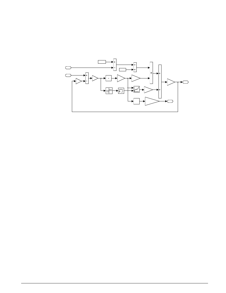
78
S
IMULINK
-S
TATEFLOW
T
ECHNICAL
E
XAMPLES
Magnetic Circuit
The model uses the applied voltage and armature position to determine the solenoid force and current.
This requires evaluating Equations 8.1 with Simulink blocks placed in the appropriate configuration. The
state variable is flux, computed by integrating the solenoid EMF. The flux density is calculated by
dividing the flux by the cross-sectional area of the magnetic path. The force F
sol
is computed as a gain
times the square of the flux density.
magnetic circuit
2
isol
1
Fsol
Lsteel
steel mmf
overall
mmf
net air gap
gmax
gap at x = 0
0.5*A/mu0
force
1/A
flux density
s
1
flux
gser
equiv. series gap
1/N
current
air mmf
u
2
H vs. B
1/mu0
R
1/N
2
vsol
1
x
armature position
Figure 8.7: Magnetic subsystem model
The model computes the solenoid current by determining the magnetomotive force. In the air gap, H
air
=
B/
µ
0
is multiplied by the gap length to give MMF
air
. The gap length is computed by subtracting the
armature position from the maximum gap. A small additional gap is added to model additional air in
the circuit, at the armature bearing surface, for example. The MMF required to produce the flux density in
the steel is computed by putting the material characteristics, H vs. B, in a 2-D lookup table. Since this
curve has significant hysteresis, two curves are placed in the table, one for increasing and one for
decreasing flux. The appropriate curve for
H
f B
steel
=
( )
is selected according to the sign of
˙
φ
. H
steel
L
steel
is added to MMF
air
and the sum is divided by N to determine the solenoid current.
Armature Motion
The model solves the equation of motion for the armature directly, as shown in Figure 8.8. The sum and
gains use standard blocks , and the subsystem Double Integrator computes the velocity and position of
the armature based on its acceleration. The position x = 0 corresponds to the maximum air gap, gmax.
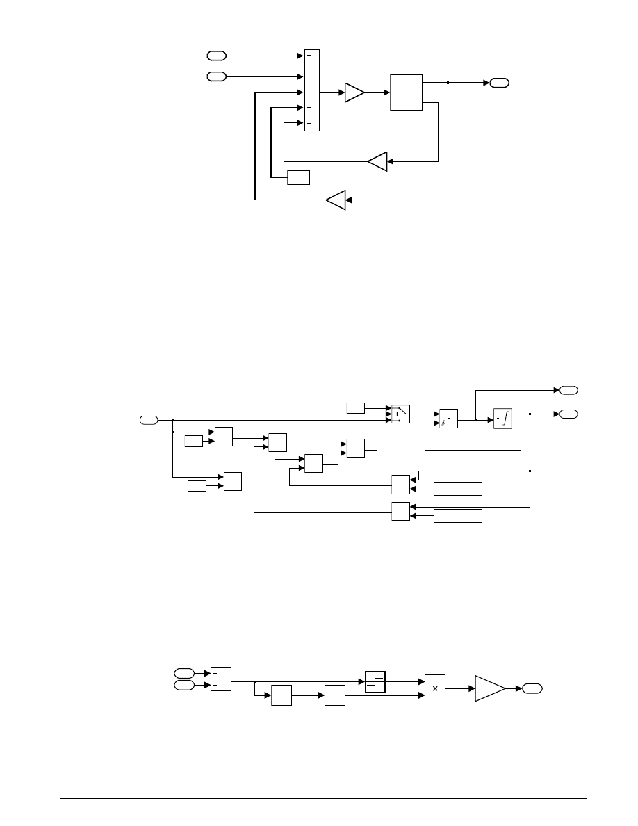
U
SING
S
IMULINK AND
S
TATEFLOW IN
A
UTOMOTIVE
A
PPLICATIONS
79
armature motion
1
stroke
Ks
spring rate
Fs0
spring preload
net force
1/m
mass
xdotdot
x
xdot
double integrator
Cv
damping
1
Fball
2
Fsol
Figure 8.8: Mechanical subsystem for the solenoid Armature
In the double integrator subsystem (Figure 8.9), the model limits the position integrator by physical stops
at x = 0 and at x = gmax - gmin (a shim typically limits the minimum gap). When these limits are
reached, it is essential that the velocity becomes zero and remains zero while at the stops. The model
achieves this by feeding the position saturation port back to the velocity reset trigger. In addition, the
derivative input of the velocity integrator switches to zero as long as xdotdot (force/mass) holds the
armature against the stop. The velocity thus remains zero until the force reverses direction.
2
xdot
1
x
Switch
<
<=
>
>=
OR
AND
AND
s
1
s
1
0
0
0
0
gmax-gmin
1
xdotdot
Figure 8.9: Cascaded integrators with c oordinated limit logic
Valve Flows
Simulink models the turbulent flow through the valve orifices with the following subsystem, shown in
Figure 8.10. The inputs pup and pdown are the upstream and downstream pressures and q is the flow
from pup to pdown. The square root of the absolute value of the pressure drop, multiplied by the sign of the
pressure drop and K
o
A
o
(defined in Equation 8.3) yields the flow.
Turbulent Orifice Flow
1
q
Ko*Ao
sqrt
|u|
2
pdown
1
pup
Figure 8.10: Individual o rifice subsystem
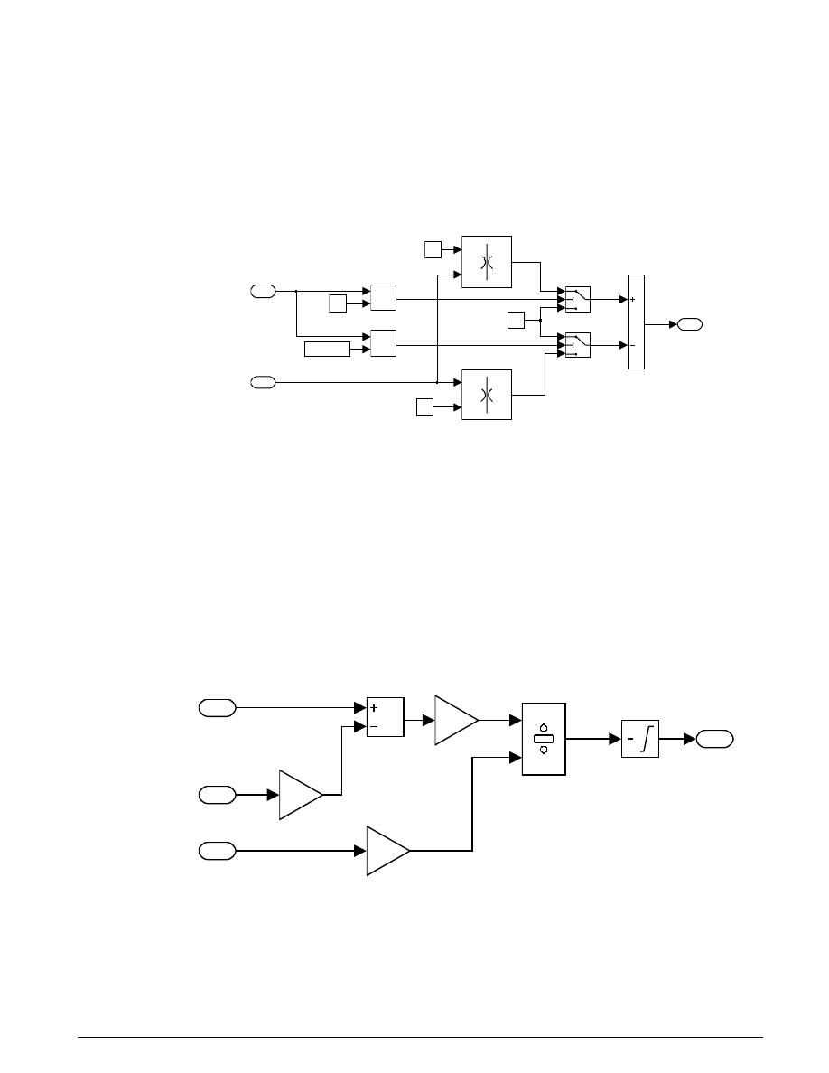
80
S
IMULINK
-S
TATEFLOW
T
ECHNICAL
E
XAMPLES
The valve model shown in Figure 8.11 uses this subsystem twice, to model the flow from the supply to the
control pressure and to model the flow from the control pressure to the exhaust. The net flow to the
control pressure is the supply flow, when x > 0, and negative one times the exhaust flow, when x <
balltravel. The maximum ball travel is less than the armature travel in order to assure that the ball seats
against the exhaust port when the armature is pulled in. During the brief time in which the ball is at
intermediate positions, with neither port blocked, flow occurs at both orifices.
poppet valve flows
1
net
flow
pup
pdown
q
source flow
pup
pdown
q
exhaust flow
>=
>
0
Ps
0
balltravel
0
2
armature position
1
control pressure
exhaust
closed
source
open
Figure 8.11: Overall v alve flow subsystem
Cylinder Pressurization
The model for cylinder pressurization is a direct realization of Equation 8.4 in the actuator dynamics
section (see Figure 8.12). Oil volume is the product of the piston position and its cross-sectional area. The
division operator uses a function block within a masked subsystem and the other blocks are standard
gains, a sum, and an integrator.
cylinder pressurization
1
pc
s
1
pressure
effective
flow
Ap
dVolume/dt
beta
bulk
modulus
Ap
Volume
3
xpdot
2
xp
1
qnet
Figure 8.12: Hydraulic c ylinder subsystem
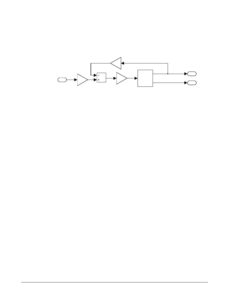
U
SING
S
IMULINK AND
S
TATEFLOW IN
A
UTOMOTIVE
A
PPLICATIONS
81
Piston Motion
Equation 8.5 is the differential equation for piston motion in the previously stated actuator dynamics
section. The Simulink implementation is straightforward, as shown in Figure 8.13. We again use the
double integrator subsystem, described above in the armature motion section, to insure that zero velocity
is indicated when the actuator is being held against its physical stops.
piston motion
2
xpdot
1
xp
Ksp
spring
1/Mp
mass
xdotdot
x
xdot
double integrator
Ap
area
1
pc
Figure 8.13: Actuator mechanical subsystem
Results
Figure 8.14 below shows the set point and piston position for a baseline simulation. During the first 0.1
second, and again from 1.0 to 1.1 seconds, the output is slew rate limited by the maximum flow available
to the actuator. At other times, the 3 Hz sinusoid is tracked closely. Although the solenoid goes through a
complete on/off cycle each PWM period, the 50 Hz dither superimposed on the actuator position is
relatively small.
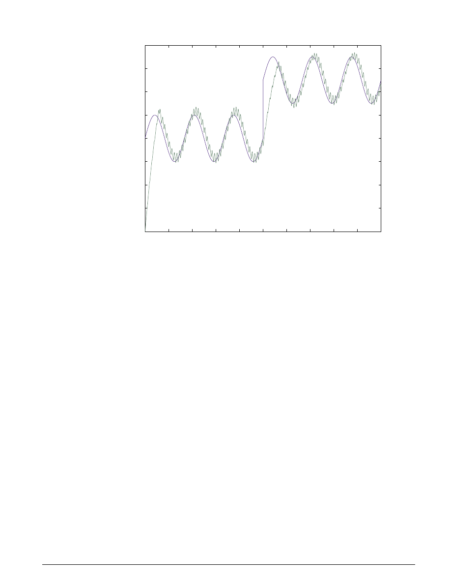
82
S
IMULINK
-S
TATEFLOW
T
ECHNICAL
E
XAMPLES
0
0.2
0.4
0.6
0.8
1
1.2
1.4
1.6
1.8
2
0.002
0.004
0.006
0.008
0.01
0.012
0.014
0.016
0.018
time (sec)
actuator position (m)
Electrohydraulic Servo Control
set point
position
Figure 8.14: Simulated p iston motion
Figure 8.15 below depicts the solenoid current control, under the authority of the Stateflow model. The
diagram shows two cycles with about 47% and about 55% duty cycle, respectively. During the pull-in
phase, as the flux builds and the current approaches its 2.5A target, the current drops abruptly at about t =
2 milliseconds. This is the instant at which the armature is pulled in. This pull-in generates so much
back EMF that the current drops appreciably. The notch in current is so distinct that it is often used in the
laboratory to measure solenoid response time.
When the current reaches the conservative 2.5A target, more than enough to achieve armature pull-in,
the solenoid enters the hold phase of its energized state. The model regulates the average current to 1A by
chopping the voltage as described in the Stateflow diagram. The chopping takes place at a rate somewhat
higher than 1 kHz in order to regulate the current within
±
0.1 A. The freewheel state uses a value of Vd =
0.5 V to slow the decay of energy in the magnetic field. When the completion of each energized state turns
off the solenoid, the negative voltage is limited by Vz = 50 V. The model achieves a rapid decay in current
without subjecting the semiconductor devices to extreme voltages.
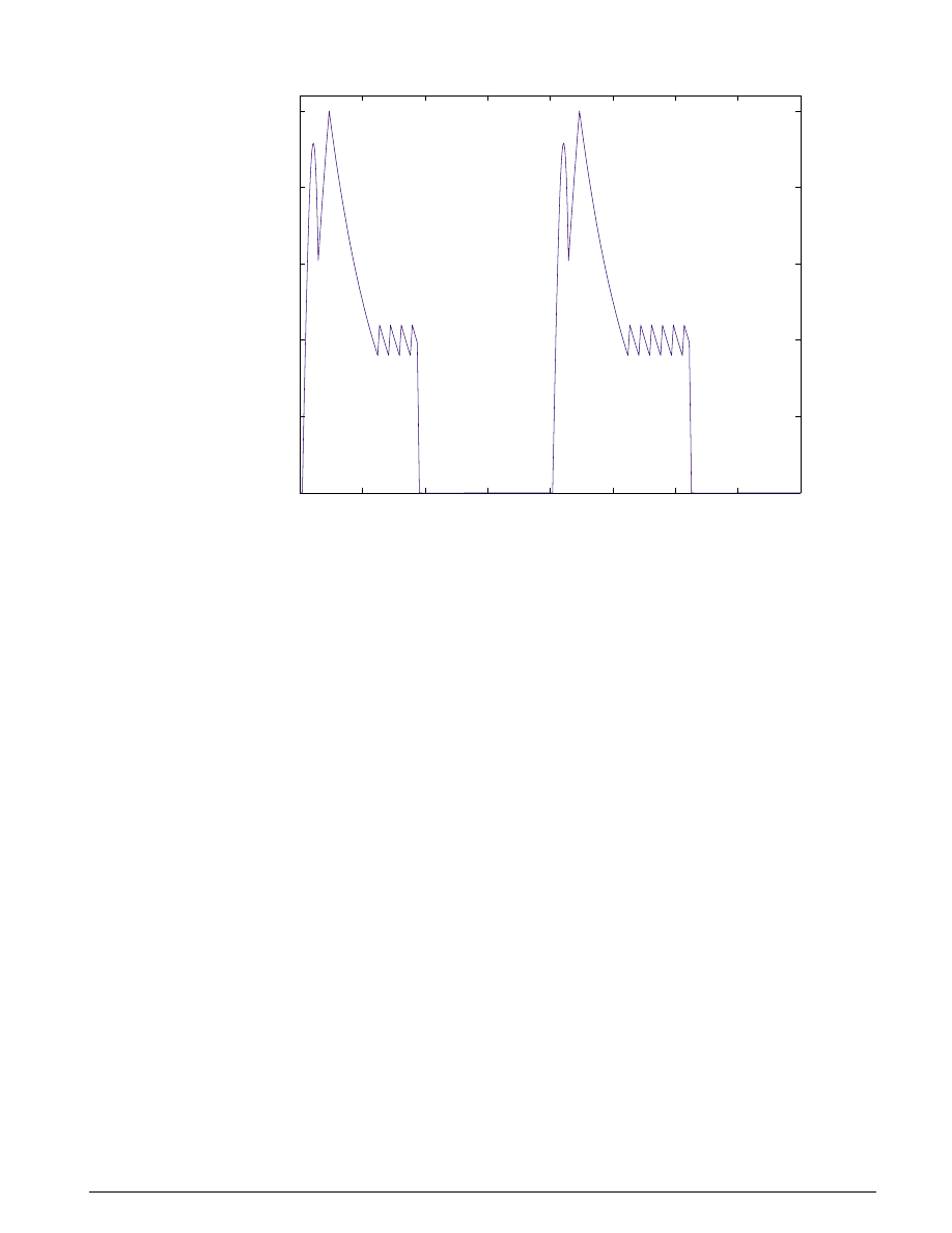
U
SING
S
IMULINK AND
S
TATEFLOW IN
A
UTOMOTIVE
A
PPLICATIONS
83
0.94
0.945
0.95
0.955
0.96
0.965
0.97
0.975
0
0.5
1
1.5
2
2.5
time (sec)
solenoid current (A)
Electrohydraulic Servo Control
PWM Driver Current Waveform
Figure 8.15: Simulated solenoid c urrent
Conclusions
Simulink and Stateflow combine to provide a powerful modeling environment for dynamic systems. In
this case, Simulink enables the direct construction of block diagram subsystems which represent the
nonlinear differential equations of the physical system and the difference equations of its discrete-time
controller. A Stateflow model captures the behavior of the electronic PWM driver circuit, without
resorting to the complexity of a detailed circuit model. The clear and natural logic of Stateflow facilitates
rapid model development and debugging. The overall model develops in a structured, hierarchical
manner, amenable to careful documentation
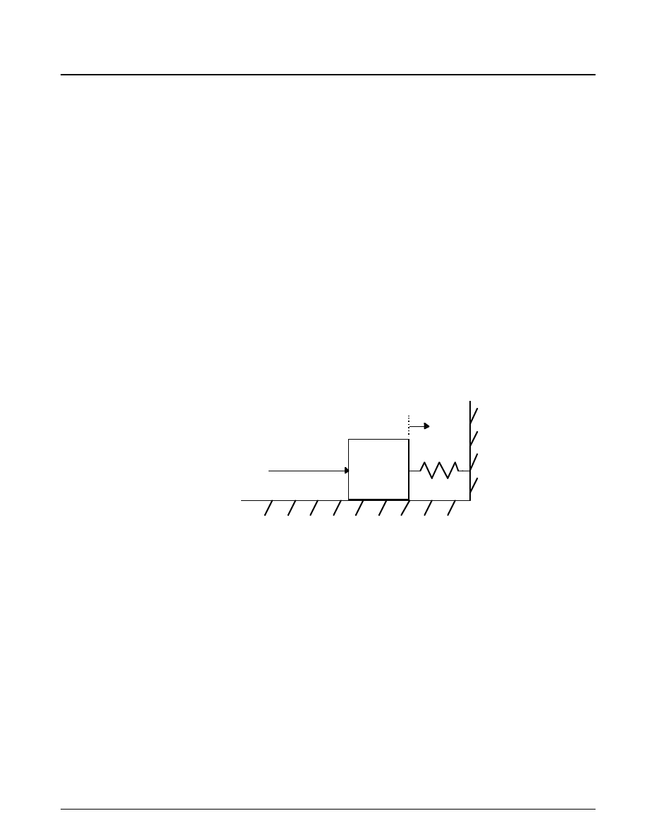
84
S
IMULINK
-S
TATEFLOW
T
ECHNICAL
E
XAMPLES
IX.
M
ODELING
S
TICK
-
S
LIP
F
RICTION
Summary
The model in this example consists of a block sliding along a surface and compressing a spring under the
influence of a user-designated input force. In the absence of friction, this behaves like a classical spring-
mass system with the steady-state block position proportional to the applied force. When friction is taken
into account, the model becomes considerably more complicated. Friction between the block and surface
tends to resist motion; however, the friction force changes with velocity and tends to be greatest when
stationary. This results in motion which alternately “sticks” and “slips” as the overall force balance
requires. This “stiction” phenomenon is common in many mechanical systems.
In this simulation, Stateflow is used to represent some of the physical states of the system. As noted above,
the friction force between two surfaces is intrinsically tied to their instantaneous relative velocity. The
continuous trajectory of velocity and position is subject to abrupt changes in acceleration, however,
corresponding to transitions between the discrete states of “stuck” and “sliding.” Simulink provides a
powerful tool for modeling the continuous dynamics, and Stateflow is a natural and intuitive setting for
modeling the discrete physical states.
Analysis and
The diagram in Figure 9.1 shows the mechanical system.
Physics
Figure 9.1: Spring-Mass-Friction System
The basic equation of motion for the block is:
Mx
F
F
F
M
x
F
in
spring
friction
in
˙˙
˙˙
=
−
−
=
=
=
block mass
acceleration
input force
Equation 9.1
The model for the linear spring (of negligible mass) is:
x
F
in
K
M

U
SING
S
IMULINK AND
S
TATEFLOW IN
A
UTOMOTIVE
A
PPLICATIONS
85
F
Kx
K
x
spring
=
=
=
spring rate
position
Equation 9.2
The friction force is more complex, however.
F
x
F
F
F
F
otherwise
x
x
velocity
x
F
F
x
friction
n
stationary
n
stationary
n
stationary
=
( )
>
=
=
=
( )
=
=
=
=
sgn ˙
,
,
,
˙
˙
˙
˙
µ
µ
µ µ
at
coefficient of friction
normal force
instantaneous force such that
0
0
Equation 9.3
In many applications the friction capacity is described by its static and kinetic magnitudes. This
approach is used in the present model, also assuming a constant normal force.
µ
µ
µ
F
F
F
x
F
F
x
n
static n
static
kinetic n
sliding
=
=
=
=
≠
,
˙
, ˙
0
0
Equation 9.4
The following logic determines F
stationary
. Whenever the velocity is nonzero, an impulsive force would be
needed to make it zero instantaneously. This always exceeds the capacity, F
sliding
, so the latter magnitude is
used. When the velocity is already zero, however, F
stationary
is the force which maintains this condition by
making the acceleration zero.
F
F
F
F
stationary
in
spring
sum
=
−
=
Equation 9.5
The friction force can thus be expressed as
F
x F
x
F
x
F
F
F
F
x
F
F
friction
sliding
sum
sum
static
sum
static
sum
static
=
≠
=
<
=
≥
sgn( ˙)
,
˙
,
˙
,
sgn(
)
, ˙
,
0
0
0
Equation 9.6
Modeling
Figure 9.2 illustrates a Simulink model that demonstrates this behavior (
sf_stickslip.mdl
). The two
main components are the block labeled
Mechanical Motion
and the block labeled
state_logic
. The former is
composed of conventional hierarchical Simulink subsystems and the latter is implemented in Stateflow.
Simulink is ideal for solving ordinary differential equations and the associated linear and nonlinear
signal flow calculations. Stateflow demonstrates its power in its ability to recognize system events which
require changes in the mode of operation.
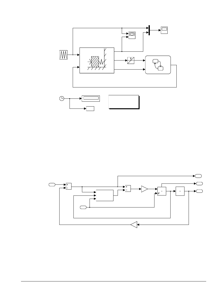
86
S
IMULINK
-S
TATEFLOW
T
ECHNICAL
E
XAMPLES
To run, choose Start from the Simulation menu.
Timekeeping
sf_stickslip.mdl
Stickslip Friction Simulation
With the default parameters, the natural
frequency is much higher than that of the
excitation force. For contrast, change
the parameter values to:
M = 0.1 kg and Fsliding = 0.1 N.
force and
position
vs. time
The input force linearly compresses
the spring, but friction resists this
movement. The magnitude of
friction depends on the state of motion.
zero threshold
novelocity
Fsum
stuck
state_logic
position
vs.
force
Fin
stuck
position
velocity
Fsum
mechanical
motion
t
edit
parameters
Mu
Mux
Input
Force
0
Figure 9.2: Simulink b lock d iagram
As described in Equation 9.2, the model implements the fundamental equation of motion, in the
Mechanical Motion block. Double-clicking on this block shows the underlying subsystem, pictured in
Figure 9.3. The sum of the forces divided by the mass determines the block acceleration. The acceleration
is integrated twice to compute the velocity and position.
Mechanical Motion
3
Fsum
2
velocity
1
position
K
spring
Fsum
xdot
stuck
Ffriction
friction force
s
1
s
1
1/M
2
stuck
1
Fin
Figure 9.3: Mechanical subsystem
The friction force subsystem shown in Figure 9.4 performs a number of nonlinear operations on the
signals in order to model the relationships of Equation 9.6. Standard Simulink blocks implement the
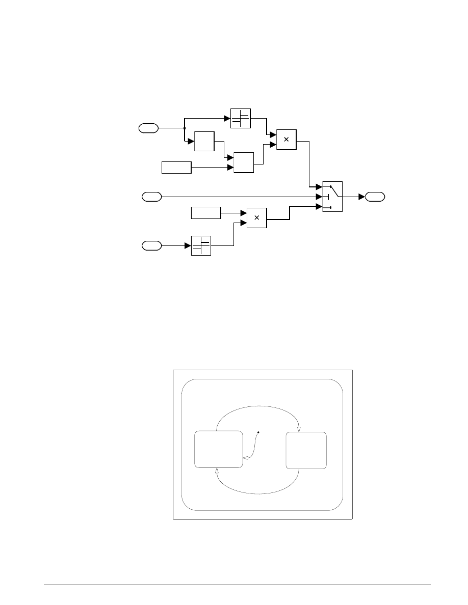
U
SING
S
IMULINK AND
S
TATEFLOW IN
A
UTOMOTIVE
A
PPLICATIONS
87
functions of absolute value, sign, minimum, and product. The switch block selects the appropriate value
for the friction force, under control of the signal labeled “stuck.” This is the output of the Stateflow
control_logic block. Note that it is also used in the
Mechanical Motion
block as a reset input to the first
integrator. This is to ensure that, at the onset of the zero velocity mode, any infinitesimal value is cleared
from the velocity state.
friction forces
fstatic
fsliding
1
Ffriction
Sign1
min
MinMax
Fstatic
Fsliding
|u|
Abs
3
stuck
2
xdot
1
Fsum
Figure 9.4: Friction Subsystem
The Stateflow diagram in Figure 9.5 below describes the behavior of the system states. The block input
signals are Fsum and novelocity. Fsum as defined in Figure 9.4 and novelocity is a binary signal that
becomes one the instant the velocity crosses through zero. The Stateflow block output is the control signal
stuck, as described above. The parameter Fstatic is taken from the M
ATLAB
workspace.
state_of_motion
stuck/
entry: stuck = 1;
sliding/
entry: stuck = 0;
[fabs(Fsum) > Fstatic]
[novelocity & (fabs(Fsum)<= Fstatic)]
state_logic
Printed 14 Nov 1997 14:52:39
Figure 9.5: Stateflow diagram for stick-slip motion

88
S
IMULINK
-S
TATEFLOW
T
ECHNICAL
E
XAMPLES
Two mutually exclusive (
OR
) states are used to represent the conditions of
stuck
and
sliding
. The
system, assumed to initially be at rest, first enters the
stuck
state via a default transition. The transition
out of the
stuck
state, the upper arc from left to right, is activated when the external forces exceed the static
friction. The
sliding
state remains active as long as the block is moving, its velocity is nonzero. When
the velocity reaches zero, its direction of travel will reverse, unless the net external force is lower in
magnitude than the static friction force. Hence, a transition from the
sliding
state to the
stuck
state is
made when the logical
and
of these two conditions, zero velocity and force less than static friction, is
satisfied.
The output signal of the machine,
stuck
, is a binary representation of the state. The entry function of the
stuck
state sets it to one, and the entry function of the
sliding
state clears it to zero. It can then be used as
a control signal in the other Simulink blocks, as indicated above. The ultimate value of the state machine
in this example is to model the state transitions of the system in accordance with physical laws while
using the appropriate frictional force in the acceleration computations at each instant.
Results
The default parameters used in this model are:
M
K
F
F
static
sliding
=
=
=
=
0 001
1
1
1
.
kg
N/m
N
N
The input force ramps linearly from zero to 5 N and back to zero, with a period of 5 seconds. Two
noteworthy characteristics of the parameters are:
1.
The natural frequency of the system
ω
n
K M
=
=
/
.
31 6
rad/sec
is much higher than that of the excitation (2
π
/10 rad/sec). As is typical in the laboratory, the model
employs a very low excitation frequency in order to determine the static response characteristics of the
system.
2.
The static and kinetic friction magnitudes are equal.
Figure 9.6 and Figure 9.7 show plots of the simulation results. Figure 9.6 shows the time histories of the
input force and the resulting position. The input force must exceed that of the static friction in order to
begin motion at t = 1. From 1 < t < 5, the position tracks the spring force less the kinetic friction force, with
small oscillations showing changes in velocity at the natural frequency
ω
n
. The input force then begins
to decrease. The mass immediately comes to a halt and sticks until t = 7, when the net force again exceeds
the static friction force, now in the reverse direction.
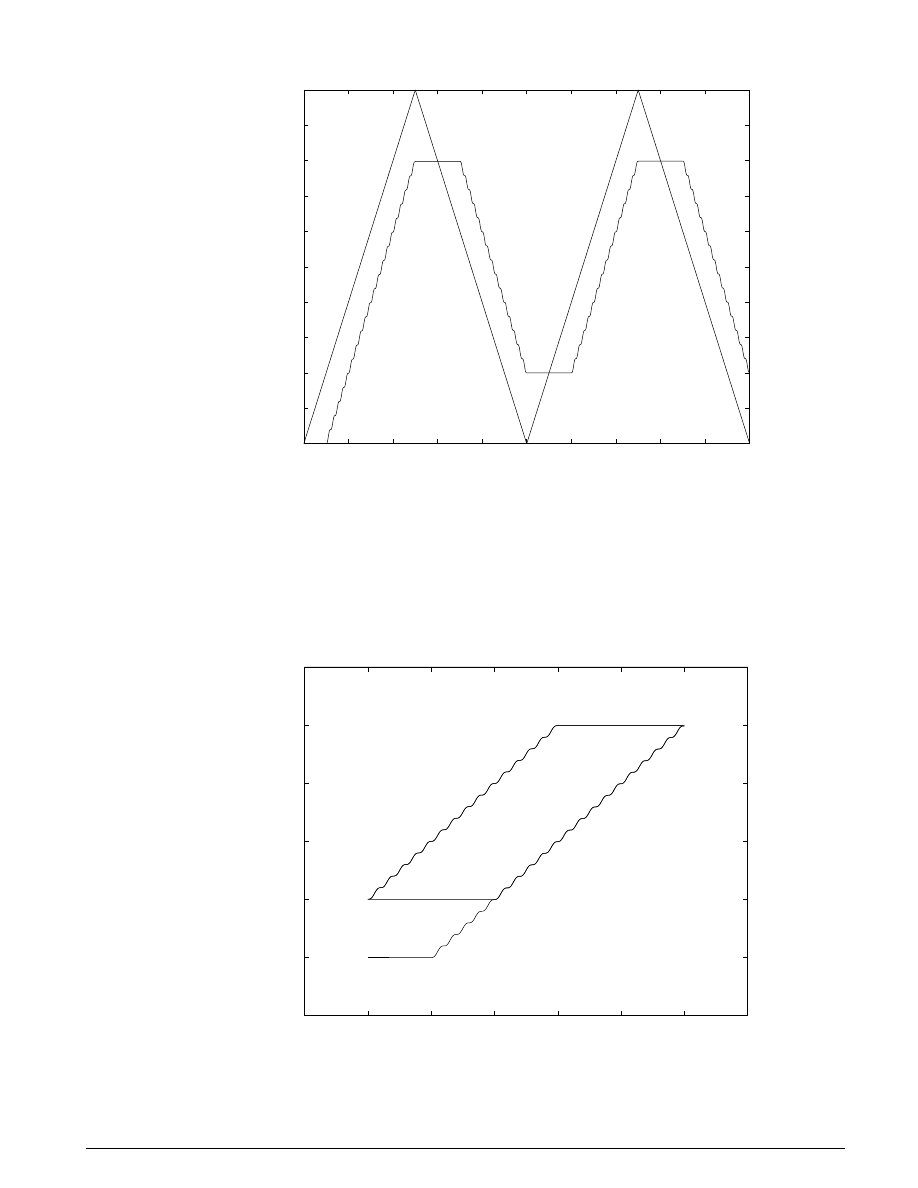
U
SING
S
IMULINK AND
S
TATEFLOW IN
A
UTOMOTIVE
A
PPLICATIONS
89
0
2
4
6
8
10
12
14
16
18
20
0
0.5
1
1.5
2
2.5
3
3.5
4
4.5
5
time (sec)
Force (N) and position (m)
Baseline Simulation
Force
Position
Figure 9.6: Simulated time histories
Similar behavior follows as the input force decreases to zero and repeats another cycle. Figure 9.7 shows
the input-output characteristics of the system, position vs. force. The plot forms a hysteresis loop as the
position lags the force. The static input-output characteristics cannot be represented by a single-valued
function because the system has memory.
-1
0
1
2
3
4
5
6
-1
0
1
2
3
4
5
force (N)
position (m)
Friction Characteristics
Figure 9.7: Simulated hysteresis loop
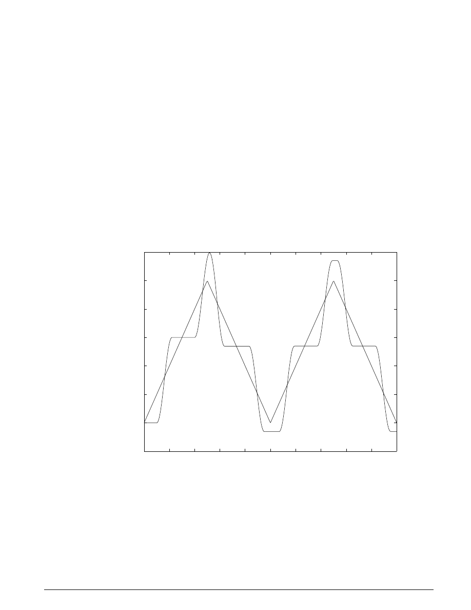
90
S
IMULINK
-S
TATEFLOW
T
ECHNICAL
E
XAMPLES
The continuous states, position and velocity, have memory in the sense that the model stores the energy
according to their magnitudes. The potential energy in the spring is proportional to the square of position
and the kinetic energy of the mass is proportional to the square of its velocity. They represent memory in
that they cannot change instantaneously if power flow is assumed to be finite.
The static behavior relies, not only on the spring rate (force vs. position), but also on the position and
velocity at the instant of the last state transition. While in the
stuck
state, the position will remain
constant at the point where it entered the state. In the
sliding
state, the position depends on the spring
characteristics, the direction of the velocity, and the position of the mass at the moment it began to slide.
This behavior is captured in a natural and intuitive way in the Stateflow model.
We can illustrate the dynamic behavior of “stiction,” or stick-slip friction, even more dramatically by
changing the system parameters as follows.
M
F
sliding
=
=
0 1
0 1
.
.
kg
N
0
2
4
6
8
10
12
14
16
18
20
-1
0
1
2
3
4
5
6
time (sec)
force (N) and position (m)
Stiction Nonlinearity
Position
Force
Figure 9.8: Stick-slip friction b ehavior
With kinetic friction lower in magnitude than static friction, abrupt discontinuities in acceleration occur
at the
stuck
-to-
sliding
and
sliding
-to-
stuck
state transitions. As the velocity reaches zero, the
acceleration is often nonzero. If the
stuck
state is entered, however, the acceleration becomes zero

U
SING
S
IMULINK AND
S
TATEFLOW IN
A
UTOMOTIVE
A
PPLICATIONS
91
immediately. This highly nonlinear behavior is typical in many systems, making it difficult to precisely
control position.
Conclusions
We can greatly simplify the modeling and simulation task by inserting a Stateflow block into the
mechanical system. Conceptually, Stateflow captures the complex dynamic nonlinear behavior in a
graphical diagram with straightforward, easy-to-read functionality. We can insert this diagram directly
into the Simulink diagram, and the tasks of code generation, compiling, and linking are seamlessly
automated to provide a powerful simulation environment.

I
NTERNATIONAL
D
ISTRIBUTORS AND
R
ESELLERS
9521v00 2/98
Contacting The MathWorks
Please send e-mail to info@mathworks.com, fax 508-647-7101, call 508-647-7000, or access our
Web site at www.mathworks.com. For address changes, please send e-mail to access@mathworks.com.
Useful e-mail addresses:
info@mathworks.com
Sales, pricing, and general information
support@mathworks.com Technical
support
access@mathworks.com
M
ATLAB
Access program information
suggest@mathworks.com
Product enhancement suggestions
resumes@mathworks.com
Resume submission for job opportunities
news-notes@mathworks.com
M
ATLAB
News & Notes Editor
updates@mathworks.com
Microcomputer updates and subscriptions
service@mathworks.com
Customer Service: order status, license renewals, passcodes
finance@mathworks.com
Financial products information
doc@mathworks.com
Documentation error reports
bugs@mathworks.com
Bug reports
connections@mathworks.com
Third-party products and services
Internet services:
www.mathworks.com
The MathWorks home page
ftp.mathworks.com
FTP server
Other resources:
comp.soft-sys.matlab
Usenet newsgroup
24 Prime Park Way
Natick, MA 01760-1500 USA
© 1998 by The MathWorks, Inc. All rights reserved. MATLAB, Simulink, Handle Graphics, and Real-Time Workshop are registered trademarks, and Stateflow and
Target Language Compiler are trademarks of The MathWorks, Inc. Other product or brand names are trademarks or registered trademarks of their respective holders.
Australia
CEANET Pty., Ltd.
Tel: +61 (0)2-9922-6311
Fax: +61 (0)2-9922-5118
E-mail: belinda@ceanet.com.au
Web: www.ceanet.com.au
Brisbane office:
Tel: +61 (0)7-3369-4499
Fax: +61 (0)7-3369-4469
E-mail: ken@ceanet.com.au
Authorized Distributors
Brazil
OpenCadd Computacao Grafica
Tel: +55-11-816-3144
Fax: +55-11-816-7864
E-mail: opencadd@sanet.com.br
Authorized Reseller
Czech Republic, Slovakia, Russia,
Ukraine, Belarus, Moldavia
Humusoft s.r.o.
Tel: +420-2-68-44-174
Fax: +420-2-68-44-174
E-mail: byron@humusoft.cz
Web: www.humusoft.cz
Authorized Reseller
France
Scientific Software Group
Tel: +33-01-41-14-67-14
Fax: +33-01-41-14-67-15
E-mail: info@ssg.fr
Web: www.ssg.fr
Authorized Distributor
Germany, Austria
Scientific Computers GmbH
Tel: +49 (0)241-470-750
Fax: +49 (0)241-449-83
E-mail: matlab.info@scientific.de
Web: www.scientific.de
Unterföhring (Munich) office:
Tel: +49 (0)89-995-901-0
Fax: +49 (0)89-995-901-11
Authorized Distributors
India, Sri Lanka
Cranes Software International (P) Ltd.
Tel: +91 (0)80-5549-338
Fax: +91 (0)80-5546-299
E-mail: matlab@CRANES.XEEBLR.
xeemail.ems.vsnl.net.in
Authorized Distributor
Israel
Omikron Delta (1927) Ltd.
Tel: +972 (0)3-561-5151
Fax: +972 (0)3-561-2962
E-mail: info@omikron.co.il
Web: www.omikron.co.il
Authorized Distributor
Italy
Teoresi s.r.l.
Tel: +39 (0)11-240-80-00
Fax: +39 (0)11-240-80-24
E-mail: info@teoresi.it
Web: www.teoresi.it
Authorized Distributor
Japan
Cybernet Systems Co., Ltd.
Tel: +81 (0)3-5978-5410
Fax: +81 (0)3-5978-5440
E-mail: infomatlab@cybernet.co.jp
Web: www.cybernet.co.jp
Authorized Distributor
Korea
Kimhua Technologies, Inc.
Tel: +82 (0)2-556-1257
Fax: +82 (0)2-556-4020
E-mail: info@soft.kimhua.co.kr
Web: kimhua.co.kr
Authorized Distributor
The Netherlands, Belgium, Luxembourg
Scientific Software Benelux B. V.
Tel: +31-(0)182-53-76-44
Fax: +31-(0)182-57-0380
E-mail: info@ssb.nl
Web: www.ssb.nl
Authorized Distributor
New Zealand
Hoare Research Software
Tel: +64-7-839-9102
Fax: +64-7-839-9103
E-mail: info@hrs.co.nz
Web: www.hrs.co.nz
Authorized Reseller
The Nordic Countries and
Baltic States
Computer Solutions Europe AB
Tel: +46 (0)8-15-30-22
Fax: +46 (0)8-15-76-35
E-mail: info@comsol.se
Web: www.comsol.se
Søborg, Denmark office:
Tel: +45 (0)39-66 56 50
Fax: +45 (0)39-66 56 20
E-mail: info@comsol.dk
Web: www.comsol.dk
Helsinki, Finland office:
Tel: +358 (0)9-455-00-55
Fax: +358 (0)9-455-00-51
E-mail: info@comsol.fi
Web: www.comsol.fi
Trondheim, Norway office:
Tel: +47 (0)735-09-220
Fax: +47 (0)735-09-221
E-mail: info@comsol.no
Web: www.comsol.no
Authorized Distributors
Poland
ControlSoft
Tel: +48 (0)12-6-17-33-48
Fax: +48 (0)12-6-33-27-12
E-mail: info@controlsoft.krakow.pl
Web: www.controlsoft.krakow.pl
Authorized Distributor
Singapore, Malaysia, Thailand,
The Philippines, Indonesia, Brunei
TechSource Systems Pte Ltd.
Tel: +65-842-4222
Fax: +65-842-5122
E-mail: info@techsource.com.sg
Authorized Distributor
South Africa
Opti-Num Solutions
Tel: +27-11-325-6238
Fax: +27-11-325-6239
E-mail: info@optinum.co.za
Web: www.optinum.co.za
Authorized Reseller
Spain, Portugal
Addlink Software Cientifico
Tel: +34 (9)3 415-49-04
Fax: +34 (9)3 415-72-68
E-mail: info@addlink.es
Web: www.addlink.es
Authorized Distributor
Switzerland
Scientific Computers SC AG
Tel: +41 (0)31-954 20 20
Fax: +41 (0)31-954 20 22
E-mail: info@scientific.ch
Authorized Distributor
Taiwan
Scientific Formosa, Inc.
Tel: +886 (0)2-2505-0525
Fax: +886 (0)2-2502-4478
E-mail: info@pent1.greenhills.com.tw
Authorized Distributor
U.K., Ireland
Cambridge Control Ltd.
Tel: +44 (0)1223-423-200
Fax: +44 (0)1223-423-289
E-mail: info@camcontrol.co.uk
Web: www.camcontrol.co.uk
Hove, England office:
Tel: +44 (0)1273-722-838
Fax: +44 (0)1273-720-550
E-mail: pauline_fox@camcontrol.co.uk
Authorized Distributors
For inquiries outside the U.S.
and Canada, please contact your
local distributor. If your country
is not listed, please contact
The MathWorks directly.
Wyszukiwarka
Podobne podstrony:
Evidence and Considerations in the Application of Chemical Peels in Skin Disorders and Aesthetic Res
Simulation for Fuel Cell Inverter using Simplorer and Simulink
L2 PAA Modelowanie układu regulacji automatycznej z wykorzystaniem pakietu MATLAB Simulink(1)
Dodatek (pakiet MATLAB z r SIMULINK)
smalec,podstawy automatyzacji L,?dania symulacyjne elementów automatyki w środowisku Matlab Simulink
Lab 3 (MATLAB SIMULINK)(W&A)
Matlab Simulink B Mrożek, Z Mrożek
Matlab Simulink sci¦ůga
Projektowanie regulatorów rozmytych w środowisku Matlab Simulink
L2 PAA Modelowanie układu regulacji automatycznej z wykorzystaniem pakietu MATLAB Simulink(1)
Matlab, Simulink Simulink Matlab to VHDL Route for Full Custom FPGA Rapid Prototyping of DSP Algori
Using Communicative Language Games in Teaching and Learning English in Primary School
83 Group tactics using sweeper and screen players in zones
MATLAB i Simulink Poradnik uzytkownika Wydanie II
MATLAB i Simulink Poradnik uzytkownika Wydanie II matsim
MATLAB & Simulink Release Notes for R2007b
MATLAB i Simulink Poradnik uzytkownika Wydanie II
więcej podobnych podstron