THERMAL CONDUCTIVITY OF

POLYMERS, GLASSES & CERAMICS BY

MODULATED DSC

S.M. Marcus and R. L. Blaine

Thermal Analysis & Rheology

ABSTRACT

This study describes a new method for the measurement of thermal conductivity of insulating materials in the range

from 0.1 to 1.5 W/

°

C m which generally covers polymers, ceramics and glasses. The method is based on Modulated

DSC and includes no modification or additions to the apparatus itself. One additional calibration step is required to

compensate for heat loss through the inert purge gas surrounding the test specimen. Best case precision is on the

order of 2% with mean values compared to literature values within 1%. While work to date includes only temperatures

near ambient, measurements above and below ambient seem possible. Further work is also currently in progress to

evaluate the applicability of this method to a broader range of materials.

INTRODUCTION

Thermal conductivity is a measure of the ease with which temperature is transmitted through a material and is a basic

material property. Materials with high thermal conductivity are called “conductors” and those with low conductivity are

called “insulators”. Solid conductors (such as metals) typically have thermal conductivities in the range of 10 to 400

W/

°

C m while insulators (such as polymers, glasses and ceramics) have values in the range of 0.1 to 2 W/

°

C m.

Furthermore, thermal conductivity changes as a weak function of temperature and rarely changes by a factor of ten

within a general class of materials.

Determination of a material’s thermal conductivity is important in evaluating its utility for specific applications. In

many of these applications, a textbook value or a single measurement near the temperature of use is sufficient to make

a decision. In a few cases, however, the material’s composition varies widely enough that regular measurement of

thermal conductivity is required. For example:

-

The manufacturers of active electronic components need to know the thermal conductivity of their encapsulat-

ing materials to be able to determine the heat dissipation of their devices. Incomplete heat dissipation may result

in the premature failure of the active element.

-

The solar energy enthusiast needs to know the thermal conductivity of the solid materials used to store the

sun’s heat energy to be able to calculate heating and cooling capacity (1).

-

Mine engineers are interested in the thermal conductivity of the rock through which they work (2). Knowl-

edge of the rock’s conductivity enables calculation of the ventilation capacity required to dissipate heat being

delivered to the mine shaft from the warm surroundings.

-

Radioactive waste management engineers need to know the thermal conductivity of the cements and grouts

used to immobilize radioactive waste since the decay steadily generates heat which must be safety dissipated (3).

-

Process and manufacturing engineers involved with the manufacture, storage, and shipping of bulk chemicals

need to know the thermal conductivity (along with several other reaction parameters) in order to predict and

eliminate potential thermal hazards.

In all of these cases (one-time measurement or on-going multiple measurements), the ability to measure thermal

conductivity easily and with modest amounts of material is useful.

THEORY

Thermal conductivity can be measured using several different instrumental techniques. One of these is based on

differential scanning calorimetry (DSC). DSC is a thermal analysis technique which measures heat flow into or out of

a material as a function of temperature or time. DSC is primarily used to measure transition temperatures and associ-

ated heats of reaction in materials, particularly polymers. Measurement of glass transition temperature, melting point,

% crystallinity, degree of cure, decomposition temperature, and oxidative stability are specific examples of some of

the more common DSC measurements.

The most widely used approach for making DSC measurements is the “heat flux” DSC, in which the sample and

reference materials (usually contained in metal pans) are placed on a thermoelectric disk inside a temperature pro-

grammed environment (Figure 1). Heat flow in this approach is measured using the thermal equivalent of Ohm’s Law

where dQ/dt = dT/R (Q = heat, t = time, T = temperature, R = thermal resistance of thermoelectric disk)(4,5). Several

researchers including Chiu (6), Sircar (7), Keating (8) and Duswalt (9) have modified heat flux DSC’s to measure the

thermal conductivity of insulating materials such as thermoplastic solids, elastomers, thermoplastic melts and pyro-

technics, respectively. In their work, a test specimen is placed in the DSC cell in contact with the sample platform.

The DSC sensor measures both the temperature of one side of the specimen and the heat flow into it. A heat sink of

known temperature is constructed to contact the opposite side of the test specimen. From the recorded heat flow and

the temperature difference between the DSC cell and the heat sink (along with the test specimen dimensions), thermal

conductivity can be calculated using the equation:

dQ/dt = -KA dT/dx

(1)

where:

Q

=

Heat (J)

t

=

Time (sec)

K

=

Thermal Conductivity (W/

°

C m)

T

=

Temperature (

°

C)

x

=

Height of test specimen (m)

A

=

Cross Sectional Area of test specimen (m2)

This DSC measurement of thermal conductivity works well but requires modification of the commercially available

DSC cell, as well as very careful attention to experimental detail. A recent extension of traditional DSC called

modulated DSC, however, minimizes those limitations.

Modulated DSC (MDSC) is a patented technique from TA Instruments in which the test specimen is exposed to a linear

heating method which has a superimposed sinusoidal oscillation (temperature modulation), resulting in a cyclic heating

profile similar to that shown in Figure 2 (solid-line). Deconvolution (separation) of the resultant experimental heat

flow during this cyclic treatment provides not only the “total” heat flow available from conventional DSC, but also

separates that total heat flow into its reversing (heat capacity related) and nonreversing (kinetic) components, thereby

providing unique insights into materials including:

•

Separation of reversing and nonreversing characteristics of thermal events (10)

•

Improved resolution of closely occurring or overlapping transitions (11,12)

•

Increased sensitivity for subtle transitions (13)

•

Direct measurement of heat capacity

It is the latter capability (direct measurement of heat capacity) which is of primary interest in this discussion because

heat capacity and thermal conductivity are related properties.

MDSC users have observed that the best heat capacity results are obtained when experimental conditions are selected

to obtain maximum temperature uniformity across the test specimen. Small, thin specimens, long oscillation periods

and complete encapsulation of the test specimen in sample pans of high conductivity (aluminum has a conductivity of

about 235 W/

°

C m) (14) produce the best results. When test conditions lie outside of these guidelines, the value of

the measured heat capacity declines. This is thought to be due to the thermal conductivity of the material preventing

uniform temperature conditions across the test specimen.

Alternatively, the effect of the specimen’s thermal conductivity may be maximized through the use of thick test

specimens and the use of open sample pans which results in the application of the temperature oscillation to only one

side of the test specimen.

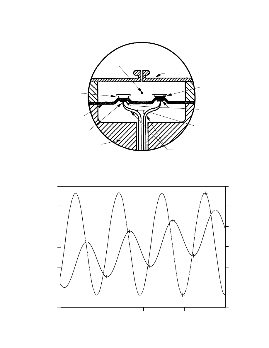
GAS PURGE

INLET

LID

SAMPLE

PAN

REFERENCE PAN

CHROMEL

DISC

ALUMEL

WIRE

THERMOELECTRIC

DISC (CONSTANTAN)

CHROMEL WIRE

THERMOCOUPLE

JUNCTION

HEATING BLOCK

Figure 1.

HEAT FLUX DSC SCHEMATIC

109

112

111

110

106

107

108

15

10

5

0

-10

-5

108.0

108.5

109.0

109.5

110.0

-15

BACKGROUND HEAT RATE 1

o

C/MIN

AMP +/- 1

o

C

PERIOD 30 SEC

-11.54

o

C

107.6

o

C

108.1

o

C

108.6

o

C

109.8

o

C

110.3

o

C

13.44

o

C/min

Modulated T

emperature

(

o

C)

[

____

.

____

] Deriv

. Modulated T

emperature (

o

C/min)

Temperature (

o

C)

Figure 2.

MDSC

TM

HEATING PROFILE

Table 1 tabulates the apparent specific heat of a series of materials comparing thin specimen encapsulated in alumi-

num sample pans/lids and a thick specimen in an open pan only. The apparent specific heat values can be quite

different under these two conditions. The difference in apparent specific heat values measured under these condi-

tions, as seen in their ratio, is greater for low thermal conductivity materials, like polystyrene and

polytetrafluoroethylene, than for the higher conductivity materials such as ceramic and glasses. The ratio for the low

conductivity polymers is about 0.44 while that for somewhat more conductive glasses and ceramics in 0.80. High

conducting aluminum samples yielded a ratio of 1.00.

Table 1

Apparent Specific Heat Capacity (J/

°

C g)

(T = 25

°

C; Amplitude = 1.0

°

C, Period = 80 s)

Material

Encapsulated

Open

Ratio

Polystyrene

1.38

0.621

0.45

Polytetrafluoroethylene

2.13

0.920

0.43

Soda Lime Glass

0.657

0.525

0.80

Pyrex® 7740 Glass

0.668

0.532

0.80

This ratio is an indication of the ease with which temperature uniformity may be achieved across the test specimen and

may be used to measure thermal conductivity.

In contrast to the steady state heat flow approach of Chiu and others mentioned previously, the modulated heat flow of

MDSC establishes a dynamic equilibrium in the test specimen permitting the measurement of thermal conductivity by

applying a cyclic temperature program to only one side of the test specimen.

The one dimensional heat flow model described in equation (1) can be expanded using the modulated heat flow

generated by the MDSC, to yield equation (2):

(dQ/dt)

2

= 2 (Z T

o

K A)

2

(2)

where:

K

=

Thermal Conductivity (W/

°

C cm)

dQ/dt =

Heat Flow Amplitude (J/sec)

ω

=

Angular Frequency (2

π

/sec)

ρ

=

Sample Density (g/(cm)

3

)

Cp

=

Sample Specific Heat (J/

°

C g)

Z

2

=

ω

ρ

Cp/(2 K)

T

o

=

Temperature Modulation Amplitude (

°

C)

L

=

Sample Length (cm)

A

=

Sample Cross Sectional Area (cm

2

)

M

=

Sample Mass (g)

C

=

Apparent Heat Capacity (J/

°

C)

Additional assumptions:

•

The specimen is a right circular cylinder with cross sectional area (A) and length (L) with parallel end

faces. The specimen has a density (

ρ

) and a specific heat (Cp).

•

The face of the specimen at the heat source follows the applied temperature modulation.

•

The heat flow through the opposing face is zero.

[

]

[

]

1 2 e

cos 2ZL + e

1 + e

cos 2ZL + e

2ZL

4ZL

2ZL

4ZL

−

•

There is no heat flow through the side of the specimen.

For materials with low thermal conductivity, the e4ZL term is large and dominates the term in brackets on the right of

the equation driving it to unity. Rearranging equation 2, noting that C = (dQ/dt) / (

ω⋅

To) and

ω

= 2

π

/Period (P), and

solving for K yields:

K = (2

π⋅

C

2

) / (Cp

ρ

A

2

P)

(3)

For a right circular cylinder,

ρ

= M/AL and A =

. Equation 3 becomes:

K = (8LC

2

) / (Cp Md

2

P)

(4)

Sample length (L), diameter (d) and mass (M) are easily measured physical parameters. The specimen’s specific heat

(Cp) may be measured using the MDSC under the optimum conditions described previously. The period (P) is an

experimental parameter. And the apparent heat capacity (C) is the measured parameter from the thermal conductivity

optimized experimental conditions.

Thus, MDSC provides all of the experimental information needed to calculate thermal conductivity.

EXPERIMENTAL

The general experimental procedure for determining thermal conductivity values at a specific temperature are de-

scribed here.

(1)

A key ingredient in any high precision measurement is securing a test specimen of uniform and

known geometry. This is also the case here. The preparation of the test specimen in the shape of a

right, circular cylinder of 6.35 mm diameter, by cutting specimens from quarter inch extruded or

molded rods, seemed to be a practical approach. Other shapes may be used but the cylinder is

convenient to machine or extrude and simplifies the measurements.

(2)

Normal calibration of the MDSC is performed using indium metal and sapphire standard reference

materials.

(3)

Thermal conductivity calibration is performed using a reference material of low and known

conductivity.

We used polystyrene specimens 0.4 and 3-4 mm in thickness and the same diameter as the unknowns.

(4)

Specific heat capacity (Cp) of the unknown material is obtained using standard MDSC procedures and

a thin (<0.5 mm) specimen.

(5)

Determine the apparent heat capacity (C) of the unknown material using a thick (>3.0 mm) test

specimen. The specimen mass, length and diameter are also measured.

Note:

The measurements in (4) and (5) are improved by putting a thin aluminum foil disk (wetted on both

sides with silicone oil) between the test specimen and the DSC measurement platform. This disk

acts to provide a more uniform heat transfer path. An equivalent foil disk with silicone oil is used

on the reference position of the cell to balance the thermal effects of the aluminum.

(6)

Using the specific heat (Cp) and apparent heat capacity thus determined, calculate the observed

thermal conductivity (Ko) using equation (4). Substituting this value, along with the thermal

conductivity calibration constant (D) into equation (6) to yield the thermal conductivity (K) of

the unknown.

In this study, four insulators were evaluated at 25

°

C using an MDSC oscillation amplitude of 1

°

C and an

oscillation period of 80 seconds.

π

d

4

2

RESULTS

Table 2 compares the values obtained by MDSC with literature values.

Table 2

Comparative Thermal Conductivities (W/

°

C m)

Without Correction for Loss Through Purge Gas

Material

Experimental

Literature Variation

Polystyrene (6, 9)

0.17

0.14

21%

Polytetrafluoroethylene (6, 9)

2.37

0.33

12%

Soda Lime Glass

0.76

0.71

7%

Pyrex® 7740 Glass (15, 16)

1.12

1.10

2%

These results show that the accuracy of the measurement declines with decreasing thermal conductivity. This is due to

a bias of about 0.03 to 0.04 W/

°

C m between the observed values and the literature values. This bias, while not large

for the higher conductivity glasses, effects the lower conductivity material by producing an appreciable deviation from

literature values.

The loss of thermal energy through the sides of the test specimen is thought to be the source of the discrepancy (bias)

in Table 2 between the thermal conductivities measured and literature values. For very low thermal conductivity

samples, such as polystyrene (K = 0.14 W/

°

C m) the thermal conductivity of the nitrogen purge gas surrounding the

test specimen (0.026 W/

°

C m) is an appreciable fraction (about one quarter) of the specimen conductivity. Hence,

under flowing purge gas conditions, the assumption of no heat flow through the sides of the sample is not strictly true.

In principle, the effect of purge gas may be reduced by the use of vacuum or low conductivity gases such as Argon,

Krypton and Xenon (0.018, 0.010, and 0.0058 W/

°

C m, respectively (17).) The use of vacuum was explored, but was

unsuccessful since it increased the noise of the measurement and therefore increased imprecision. Its use was

abandoned. The use of low conductivity purge gases was not pursued in this study because a calibration approach

described in the following paragraphs was developed and was found to be accurate and precise.

Modeling the premise of heat loss though the sides of the test specimen creates a thermal conductivity calibration

constant (D) which may be used to correct for this effect. The value for D is obtained using a calibration material of

low thermal conductivity (e.g. polystyrene), and equation (5):

D = (K

o

.

K

r

)

0.5

- K

r

(5)

where:

D

=

Thermal Conductivity Calibration Constant

K

o

=

Observed Reference Material Thermal Conductivity (W/

°

C m)

K

r

=

True Reference Material Thermal Conductivity (W/

°

C m)

For 6.35 mm diameter test specimens, the value for D is typically 0.014 W/

°

C m. This value may then be substituted

into equation (6) to obtain the thermal conductivity of unknown specimens.

K = [K

o

- 2D + (K

o2

- 4DK

o

)

0.5

] / 2

(6)

where, K

o

now is the observed conductivity of the unknown specimen.

Using the determined value of the thermal conductivity calibration constant and equation (6), the values in Table 2 are

upgraded to the values presented in Table 3:

Table 3

Comparative Thermal Conductivities (W/oC m)

With correction for Loss Through Purge Gas

Material

Experimental

Literature Variation

Polystyrene

0.14

0.14

0%

Polytetrafluoroethylene

0.34

0.33

3%

Soda Lime Glass

0.73

0.71

3%

Pyrex® 7740

1.09

1.10

1%

The accuracy of any method for the measurement of thermal conductivity is dependent upon the availability of refer-

ence materials with which a comparison may be made. Pyrex



7740 is one of the few materials which may serve as a

standard reference material since it has been well tested by the National Institute for Standards and Technology (NIST)

(16). As Table 3 indicates, the accuracy of this approach for Pyrex



7740 is about 1% using the mean value of

triplicate determinations. The literature values in Table 3 for the other materials evaluated represent those generally

reported (6,9). In all cases, the MDSC determined values agreed within about 3%.

The precision of MDSC thermal conductivity measurements can be estimated by treating equation (3) using the

principle of propagation of uncertainties to obtain:

(7)

where the differential values represent the percent uncertainty in the individual measurements. Since mass (M), length

(L), period (P), diameter and area (A) can all be determined with precision <0.1%, the precision of the thermal

conductivity measurement is dominated by the precision of the apparent heating capacity and specific heat determina-

tions. dCp/Cp is estimated to be ca. 1% so the thermal conductivity precision should be 3-4%. This estimation is

confirmed by experimental results presented in Table 4. The pooled coefficient of variation of the 4 measurements is

4.7%.

Table 4

Precision

Material

Mean (W/°Cm)

Coef. Var. (%)

Polystyrene

0.14

2.2

Polytetrafluoroethylene

0.34

2.3

Soda Lime Glass

0.73

7.5

Pyrex® 7740

1.09

4.7

Chiu and his co-workers estimated the precision of their DSC approach to be about 3%, and others have estimated its

accuracy at about 5%. Duswalt has made considerable improvement in this approach using a ratio method comparing

experimental results with those for a reference material of known value (9). ASTM Test method E1225 estimates

precision at 7%, and D4351 shows repeatability (precision) values on the order of 5.6%. Reproducibility values of

11% are obtained when applied to polymers (18).

The ratio method of Duswalt was used as a reference with which the results of the MDSC approach were compared.

Duswalt’s value for these same test specimens are those presented as literature values in Table 3 for polystyrene and

polytetrafluoroethylene.

Thus the approach described here appears to provide accuracy and precision at least equivalent to other methods in

common use for insulators without the necessity for a specialized apparatus.

dK / K = 3 dCp / Cp + dM / M + dA / A + dL / L + dP

P

REFERENCES

1.

Irby, R.G., J.R. Parsons and E.G. Keshock, Thermal Conductivity 19,

D.W. Yarbrough (ed.), Plenum Press, 121-143 (1988).

2.

Ashworth, T. and D.R. Smith, Thermal Conductivity 19, D.W. Yarbrough (ed.).,

Plenum Press, 145-153 (1988).

3.

Gilliam, T.M., and I.L. Morgan, Thermal Conductivity 19, D.W. Yarbrough (ed.),

Plenum Press, 93-108 (1988).

4.

Thermal Analysis Review: Generic Definition for DSC, TA Instruments

Publication TA 081.

5.

ASTM Test Method E1225 “Thermal Conductivity of Solids by Means of the

Guarded-Comparative-Longitudinal Heat Flow Technique”, Annual Book of

ASTM Standards, Vol. 14.02.

6.

Chiu, J. and P.G. Fair, Thermochim. Acta, 34, 267-273 (1979).

7.

Sircar, A.K. and J.L. Wells, Rubb. Chem. Tech., 54, 191-207 (1982).

8.

Keating, M.Y. and C.S. McLaren, Thermochim. Acta, 166, 69-76 (1990).

9.

Duswalt, A.A., 48th Calorimeter Conference, Durham NC, (1993)

10.

TA Instruments Publication MDSC 1

11.

TA Instruments Publication MDSC 2

12.

TA Instruments Publication TA 074

13.

TA Instruments Publication MDSC 3

14.

Gray, D.W. (ed.), American Institute of Physics Handbook, 3rd edition, pages 4-

143 to 4-162 (1982).

15.

Powell, R.W., C.Y. Ho and P.E. Liley, Thermal Conductivity of Selected Materials,

NSRDS-NBS8, National Bureau of Standards Reference Data Series (1966).

16.

Hulstrom, L.C., Thermal Conductivity 19, D.W. Yarbrough (ed.), Plenum Press,

199-211 (1988).

17.

Perry, R.H., D.W. Green and J.O. Maloney, Perry’s Chemical Engineers’

Handbook, Sixth Edition, McGraw-Hill, 3-254 (1984).

18.

ASTM Test Method D4351 “Thermal Conductivity of Plastics by the Evaporation-

Calorimetric Method”, Annual Book of ASTM Standards, Vol. 8.03.

TA-086