A Hybrid Model to Detect Malicious Executables

Mohammad M. Masud

Latifur Khan

Bhavani Thuraisingham

Department of Computer Science

The University of Texas at Dallas

Richardson, TX 75083-0688

{mehedy, lkhan, bhavani.thuraisingham}@utdallas.edu

Abstract— We present a hybrid data mining approach to detect
malicious executables. In this approach we identify important
features of the malicious and benign executables. These features
are used by a classifier to learn a classification model that can
distinguish between malicious and benign executables. We
construct a novel combination of three different kinds of
features: binary n-grams, assembly n-grams, and library function
calls. Binary features are extracted from the binary executables,
whereas assembly features are extracted from the disassembled
executables. The function call features are extracted from the
program headers. We also propose an efficient and scalable
feature extraction technique. We apply our model on a large
corpus of real benign and malicious executables. We extract the
abovementioned features from the data and train a classifier
using Support Vector Machine. This classifier achieves a very
high accuracy and low false positive rate in detecting malicious
executables. Our model is compared with other feature-based
approaches, and found to be more efficient in terms of detection
accuracy and false alarm rate.

Keywords- disassembly, feature extraction, malicious

executable, n-gram analysis.

I.

I

NTRODUCTION

Malicious code is a great threat to computers and computer

society. Numerous kinds of malicious code wander in the wild.

Some of them are mobile, such as worms, and spread through

the internet crashing thousands of computers worldwide. Other

kinds of malicious code are static, like viruses, but sometimes

deadlier than its mobile counterpart. Malicious code writers

mainly exploit different kind of software vulnerabilities to

attack host machines. There has been tremendous effort

imparted by researchers to counter the attacks of malicious

code writers. Unfortunately, the more successful the

researchers become in cracking down malicious code, the more

sophisticated mal-code appear in the wild, evading all kinds of

detection mechanisms. Thus, the battle between malicious code

writers and researchers is virtually a never-ending game.

Although signature based detection techniques are being

used widely, they are not effective against “zero-day attacks”

and various “obfuscation” techniques. Signature based

technique is also hopeless against new attacks. So, there has

been a growing need for fast, automated, and efficient detection

technique that can also detect new attacks. Many automated

systems [1-8] have already been developed by different

researchers in recent years.

In this paper we describe our new model, the Hybrid

Feature Retrieval (HFR) model, which can detect malicious

executables efficiently. Our model extracts three different kinds

of features from the executables and combines them into one

feature set, which we call the hybrid feature set (HFS). These

features are used to train a classifier using Support Vector

Machine (SVM). This classifier is then used to detect malicious

executables. The features that we extract are: i) binary features,

ii) derived assembly features and iii) dynamic link library

(DLL) call features. The binary features are extracted as binary

n-grams (i.e., n consecutive bytes) from the binary executable

files. This extraction process is explained in section III (A).

Derived assembly features are extracted from disassembled

executables. A derived assembly feature is actually a sequence

of one or more assembly instructions. We extract these features

using our sophisticated assembly feature retrieval (AFR)

algorithm, explained in section IV (B). These derived assembly

features are similar to, but not exactly the same as assembly n-

gram features (explained in section III (B)). We do not directly

use the assembly n-grams features in HFS, because we observe

during our initial experiments [9] that derived assembly

features perform better than assembly n-gram features. The

process of extracting derived assembly features is not trivial,

but involves a lot of technical challenges. It is explained in

section IV. DLL call features are also extracted from the header

of the disassembled binaries, and explained elaborately in

section III (C). We show empirically that the combination of

these three features is always better than any single feature in

terms of classification accuracy. We discuss our results in

section V.

Our contributions to this research work are as follows. First,

we propose and implement our HFR model, which combines

three types of features mentioned above. Second, we apply a

novel idea to extract assembly features using binary features. A

binary feature or binary n-gram may represent an assembly

instruction, or part of one or more instructions, or even a string

data inside the code block. Thus, a binary n-gram may

represent some partial information. But we apply AFR

algorithm to retrieve the most appropriate assembly instruction

or instruction sequences corresponding to the binary n-gram.

We call it the most appropriate assembly instruction sequence

because there may be multiple possible assembly instruction

sequences corresponding to a single binary n-gram, and AFR

selects the most appropriate of them by applying some

selection criteria. If the binary n-gram represents a partial

assembly instruction or instruction sequence, then we find the

U.S. Government work not protected by U.S. Copyright

This full text paper was peer reviewed at the direction of IEEE Communications Society subject matter experts for publication in the ICC 2007 proceedings.

corresponding complete instruction sequence, and use this as a

feature. The net effect is that, we convert a binary feature to an

assembly feature. We hope that the assembly feature would

carry more complete and meaningful information than the

binary feature. Third, we propose and implement a scalable

solution to the n-gram feature extraction and selection problem

in general. Our solution not only solves the limited memory

problem but also applies efficient and powerful data structures

to ensure fast running time. Thus, it is scalable to very large set

of executables (in the order of thousands), even with limited

main memory and processor speed. Fourth, we compare our

results with a recently published work [10] that is claimed to

have achieved high accuracy using only binary n-gram feature,

and we show that our method is superior to that.

The rest of the paper is organized as follows: Section II

discusses related works, Section III presents and explains

different kinds of n-gram feature extraction methods, Section

IV describes the HFR model, Section V discusses our

experiments and analyzes results, Section VI concludes with

future research directions.

II. RELATED

WORK

There has been a significant amount of research in recent

years to detect malicious executables. Researchers apply

different approaches to automate the detection process. One of

them is behavioral approach, which is mainly applied to mobile

malicious code. Behavioral approaches try to analyze

characteristics such as source and destination addresses, build

statistical models of packet flow at the network level, consider

email attachments etc. Examples of behavioral approaches are

social network analysis [1, 2], and statistical analysis [3]. A

data mining based behavioral approach for detecting email

worms as been proposed by Masud et al. [4].

Another approach is content-based, which analyzes the

content of the code. Some content based approaches try to

generate signature automatically from network packets.

Examples are EarlyBird [5], Autograph [6], and Polygraph [7].

Another kind of content-based approach extracts features from

the executables and apply machine learning to classify

malicious executables. Stolfo et al. [8] extract DLL call

information using GNU Bin-Utils [11], and character strings

using GNU strings, from the header of Windows PE

executables. Also, they use byte sequences as features. They

report accuracy of their features using different classifiers.

A similar work is done by Maloof et al. [10]. They extract

binary n-gram features from the binary executables and apply

them to different classification methods, and report accuracy.

Our model is also content based. But it is different from [10] in

that it extracts not only the binary n-grams but also assembly

instruction sequences from the disassembled executables, and

gathers DLL call information from the program headers. We

compare our model’s performance with [10], since they report

higher accuracy than [8].

III. F

EATURE

E

XTRACTION USING N

-

GRAM

A

NALYSIS

Feature extraction using n-gram analysis involves

extracting all possible n-grams from the given dataset (training

set), and selecting the best n-grams among them. We extend

the notion of n-gram from bytes to assembly instructions, and

to DLL function calls. That is, an n-gram may be either a

sequence of n bytes or n assembly instructions, or n DLL

function calls, depending on whether we want to extract

features from binary or assembly program, or DLL call list.

Before extracting n-grams, we preprocess the binary

executables by converting them to hexdump files and assembly

program files, as explained below.

A. Binary n-gram feature

We apply the UNIX hexdump utility to convert the binary

files into text files (‘hexdump’ files), containing the

hexadecimal number corresponding to each byte of the binary

file. The feature extraction process consists of two phases: i)

feature collection, and ii) feature selection, both of which are

explained in subsequent paragraphs.

1) Feature Collection

We collect n-grams from the ‘hexdump’ files. As an

example, the 4-grams corresponding to the 6 bytes sequence

“a1b2c3d4e5f6” are “a1b2c3d4”, “b2c3d4e5” and “c3d4e5f6”,

where “a1”,”b2”,…etc are the hexadecimal representation of

each byte.

N-gram collection is done in the following way: we scan

through each file by sliding a window of n bytes. If we get a

new n-byte sequence, then we add it to a list, otherwise we

discard it. In this way, we gather all the n-grams. But there are

several implementation issues related to the feature collection

process. First, the total number of n-grams is very large. For

example, the total number of 10-grams in ‘dataset2’ (see

Section V(A)) is 200 million. It is not possible to store all of

them in computer’s main memory. Second, each newly

scanned n-gram must be checked against the list. This requires

a search through the entire list. If a linear search is performed,

it will take a long time to collect all the n-grams. The total time

for collecting all n-grams would be O (N

2

), where N is the total

number of n-grams, which is very large when N=200 million.

In order to solve the first problem, we use disk I/O. We

store the n-grams in the disk in sorted order to enable merging

with the n-grams in the main memory.

In order to solve the second problem, we use a data

structure called Adelson Velsky Landis (AVL) tree [12] to

store the n-grams in memory. An AVL tree is a height-

balanced binary search tree. This tree has a property that the

absolute difference between the heights of the left sub-tree and

the right sub-tree of any node is at most one. If this property is

violated during insertion or deletion, a balancing operation is

performed and the tree regains its height-balanced property. It

is guaranteed that insertions and deletions are performed in

logarithmic time. So, in order to insert an n-gram in memory,

we now need only O (log

2

(N)) searches. So, the total running

time is reduced to O (Nlog

2

(N)) from O (N

2

), which is a great

improvement for N as large as 200 million.

2) Feature Selection

Since the number of extracted features is very large, it is not

possible to use all of them for training because of the following

reasons. First, the memory requirement would be impractical.

This full text paper was peer reviewed at the direction of IEEE Communications Society subject matter experts for publication in the ICC 2007 proceedings.

Second, training time of any classifier would be too long.

Third, a classifier would be confused with such a large number

of features, because most of the features would be noisy,

redundant or irrelevant. So, we are to choose a small, relevant

and useful feature set from the very large set. We choose

information gain as the selection criterion, because it is one of

the best criteria used in literature for selecting the best features

from.

Information gain can be defined as a measure of the

effectiveness of an attribute (i.e., feature) in classifying the

training data [13]. If we split the training data on this attribute

values, then information gain gives the measurement of the

expected reduction in entropy after the split. The more an

attribute can reduce entropy in the training data, the better the

attribute in classifying the data. Information Gain of an

attribute A on a collection of examples S is given by (1):

∑

∈

−

≡

)

(

)

(

|

|

|

|

)

(

)

,

(

A

Values

V

v

v

S

Entropy

S

S

S

Entropy

A

S

Gain

… (1)

Where Values(A) is the set of all possible values for

attribute A, and S

v

is the subset of S for which attribute A has

value v. In our case, each attribute has only two possible values

(0, 1). If this attribute is present in an instance (i.e., executable)

then the value of this attribute for that instance is 1, otherwise it

is 0. Entropy of S is computed using the following equation (2):

)

)

(

)

(

)

(

(

log

)

(

)

(

)

(

)

)

(

)

(

)

(

(

log

)

(

)

(

)

(

)

(

2

2

s

p

s

n

s

n

s

p

s

n

s

n

s

p

s

n

s

p

s

p

s

n

s

p

S

Entropy

+

+

−

+

+

−

=

… (2)

Where p(S) is the number of positive instances in S and n(S)

is the total number of negative instances in S. We denote the

best 500 features, selected using information gain criterion, as

the Binary Feature Set (BFS). We generate feature vectors

corresponding to the BFS for all the instances in the training

set. A feature vector corresponding to an instance (i.e., an

executable) is a binary vector having exactly one bit for each

feature, and a bit is ‘one’ if the corresponding feature is present

in the example and ‘zero’ otherwise. Feature vectors are used

to train classifier with SVM.

B. Assembly n-gram feature

We disassemble all the binary files using a disassembly tool

called PEDisassem [14] that is used to disassemble Windows

Portable Executable (P.E.) files. Besides generating the

assembly instructions with opcode and address information,

PEDisassem provides useful information like list of resources

(e.g. cursor) used, list of DLL functions called, list of exported

functions, and list of strings inside the code block and so on.

In order to extract assembly n-gram features, we follow a

method very similar to the binary n-gram feature extraction.

First we collect all possible n-grams, i.e., sequence of n

instructions, and select best 500 of them according to

information gain. We call this selected set of features as

Assembly Feature Set (AFS). We face the same difficulties of

limited memory and long running time as in byte n-grams, and

solve them in the same way.

As an example of assembly n-gram feature extraction,

assume that we have a sequence of 3 instructions:

“push eax”; “mov eax, dword[0f34]” ; “add ecx, eax”;

and that want to extract all the 2-grams, which are:

(1) “push eax”; “mov eax, dword[0f34]”;

and (2) “mov eax, dword[0f34]”; “add ecx, eax”;

We adopt a standard representation of assembly

instructions, which has the following format:

name.param1.param2, where name is the instruction name

(e.g., mov), param1 is the first parameter, and param2 is the

second parameter. Again, a parameter is any one of the

followings {register, memory, constant}. So, the second

instruction in the above example: “mov eax, dword[0f34]”,

after standardization, becomes: “mov.register.memory”.

We also compute binary feature vectors for the AFS. Please

note that we do not use the AFS in our HFS. We use AFS only

for comparison purposes.

C. DLL function call feature

We extract information about DLL function calls made by a

program by parsing the disassembled file. We define the n-

gram of DLL function call as a sequence of n DLL calls that

appears in the disassembled file. For example, assume that the

disassembled file has the following sequence of instructions

(omitting all instructions except DLL calls):

“…”

+

; “call KERNEL32.

LoadResource

”; “…”; “call

USER32.

TranslateMessage

”; “…”; “call USER32.

DispatchMessageA

”

+

(0 or more instructions other than DLL call)

The 2-grams would be:

(1) “

KERNEL32.

LoadResource,

USER32.

TranslateMessage”

and (2)“

USER32.

TranslateMessage,

USER32.

DispatchMessageA ”

After extracting the n-grams we select best 500 of them

using information gain. We then generate the feature vectors in

a similar way as explained earlier. We also compute binary

feature vector for the selected DLL call features.

IV. T

HE

H

YBRID

F

EATURE

R

ETRIEVAL

M

ODEL

The Hybrid Feature Retrieval (HFR) Model is illustrated in

fig. 1. It consists of different phases and components. Most of

the components have already been discussed in details. Below

is a brief description of the model.

A. Description of the Model

The Hybrid Feature Retrieval (HFR) Model consists of two

phases: the training phase and the testing phase. The training

phase is shown in Figure 1(a), and testing phase is shown in

Figure 1(b).

This full text paper was peer reviewed at the direction of IEEE Communications Society subject matter experts for publication in the ICC 2007 proceedings.

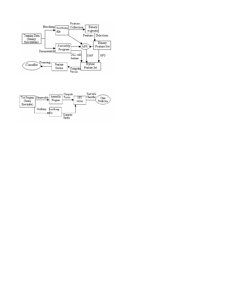
Figure 1(a). The Hybrid Feature Retrieval Model, training phase.

Figure 1(b). The Hybrid Feature Retrieval Model, testing phase.

In the training phase we convert binary executables into

hexdump files and Assembly Program files using UNIX Hex-

dump utility and the disassembly tool PEDisassem,

respectively. We extract binary n-gram features using the

approach explained in section III (A). We then apply AFR

algorithm (to be explained shortly) to retrieve assembly

instruction sequences, called the derived assembly features

(DAF), that best represent the selected binary n-gram features.

We combine these features with the DLL function call features,

and denote this combined feature set as Hybrid Feature Set

(HFS). We compute the binary feature vector corresponding to

the HFS and train a classifier using SVM. In the testing phase,

we scan the test file and compute the feature vector

corresponding to the HFS. This vector is tested against the

classifier. The classifier outputs the class prediction {benign,

malicious} of the test file.

The main challenge that we face is that of finding DAF

using the binary n-gram features. The main reason for finding

DAF is that we observe that a binary feature may sometimes

represent partial information. For example: it may represent

part of one or more assembly instructions. Thus, a binary

feature is sometimes a partial feature. We would like to find

the complete feature corresponding to the partial one, which

represents one or more whole instructions. We then use this

complete feature instead of the partial feature so that we can

obtain a more useful feature set.

B. The Assembly Feature Retrieval (AFR) algorithm

The AFR algorithm is used to extract derived assembly

instruction sequences (i.e., DAF) corresponding to the binary

n-gram features. As we have explained earlier, we do not use

assembly n-gram features (AFS) in the HFS, because we

observe that AFS performs poorer compared to DAF. Now we

describe the problem with some examples and then explain

how it has been solved.

The problem is: given a binary n-gram feature, how to find

its corresponding assembly code. The code should be searched

through all the assembly programs files. The solution consists

of several steps.

First, we apply our linear address matching technique: we

use the offset address of the n-gram in the binary file to look

for instructions at the same offset at the assembly program file.

Based on the offset value, one of the three situations may

occur:

i. The offset is before program entry point, so there is no

corresponding code for the n-gram. We refer to this address as

Address Before Entry Point (ABEP).

ii. There is some data, but no code at that offset. We refer to

this address as DATA.

iii. There is some code at that offset. We refer to this

address as CODE.

Second, we select the best CODE instance among all

instances. We apply a heuristic to find the best sequence, which

we call the Most Distinguishing Instruction Sequence (MDIS)

heuristic. According to this heuristic, we choose the instruction

sequence that has the highest information gain. Due to the

shortage of space, we are unable to explain details of our

algorithm here. Please refer to [9] for a detailed explanation

with examples of the AFR algorithm, and MDIS heuristics.

V. E

XPERIMENTS

We design our experiments to run on two different datasets.

Each dataset has different sizes and distributions of benign and

malicious executables. We generate all kinds of n-gram

features (e.g. binary, assembly, DLL) using the techniques

explained in section III. We also generate the HFS (see section

IV) using our model. We test the accuracy of each of the

feature sets using SVM, applying a three-fold cross validation.

We use the raw SVM output (i.e., probability distribution) to

compute the average accuracy, false positive and false negative

rate, and Receiver Operating Characteristic (ROC) graphs

(using techniques in [15]).

A. Dataset

We have two non-disjoint datasets. The first dataset

(dataset1) contains a collection of 1,435 executables, 597 of

which are benign and 838 are malicious. The second dataset

(dataset2) contains 2,452 executables, with 1,370 benign and

1,082 malicious. So, the distribution of dataset1 is

benign=41.6%, malicious=58.4%, and that of dataset2 is

benign=55.9%, malicious=44.1%. We collect the benign

executables from different Windows XP, and Windows 2000

machines, and collect the malicious executables from [16],

which contains a large collection of malicious executables. We

select only the Win32 executables in both cases. We would like

to experiment with the ELF executables in future.

This full text paper was peer reviewed at the direction of IEEE Communications Society subject matter experts for publication in the ICC 2007 proceedings.

B. Experimental setup

Our implementation is developed in Java with JDK 1.5. We

use the libSVM library [17] for SVM. We run C-SVC with a

Polynomial kernel, gamma = 0.1, and epsilon = 1.0E-12. Most

of our experiments are run on two machines: a Sun Solaris

machine with 4GB main memory and 2GHz clock speed, and a

LINUX machine with 2GB main memory and 1.8GHz clock

speed. The disassembly and hex-dump are done only once for

all machine executables and the resulting files are stored. We

then run our experiments on the stored files.

C. Results

We first present classification accuracies, and the Area

Under the ROC Curve (AUC) of different methods in Table-I,

and Table-II respectively, for both datasets and different values

of n.

From Table-I we see that the classification accuracy of our

model is always better than other models, on both datasets. On

dataset1, the best accuracy of the hybrid model is for n=6,

which is 97.4, and it is 1.9% higher than BFS. On average,

HFS’s accuracy is 6.5% higher than BFS. Accuracy of AFS is

always the lowest, and much lower than the other two. The

average accuracy of AFS is 10.3% lower than HFS. The reason

behind this poor performance is that Assembly features

consider only the CODE (see IV-B) part of the executables. If

any code is encrypted as data, it cannot be decrypted by our

disassembly tool, and thus the whole encrypted portion is

recognized as DATA and ignored by our feature extractor.

Thus, AFS misses a lot of information and consequently the

extracted features also have poorer performance. But BFS

considers all parts of the executable and thus able to detect

patterns from encrypted parts too. If we look at the accuracies

of dataset2, we find that the difference between the accuracies

of HFS and BFS is greater than that of dataset1. For example,

the average accuracy of HFS is 8.6% higher. AFS again

performs much poorer than the other two. It is interesting to

note that HFS has an improved performance over BFS (and

AFS) in dataset2, which has more benign examples than

malicious. This is more likely in real world; we have a lot

more benign examples than malicious ones. This implies that

our model will perform much better in a real-world scenario,

having larger number of benign executables in the dataset. One

interesting observation from table-I is that accuracy for 1-gram

BFS is very low. This is because a 1-gram is only a 1-byte long

pattern, which is not long enough to be useful.

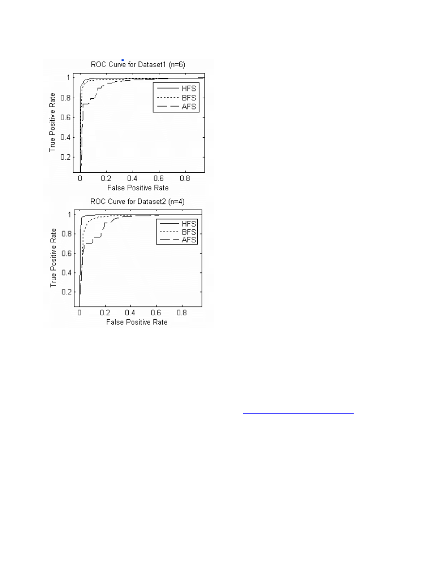
Figure 2 shows ROC curves of dataset1 for n=6 and

dataset2 for n = 4. Note that ROC curves for other values of n

have similar trends, except n = 1, where AFS performs better

than BFS. It is evident from the curves that HFS is always

dominant over the other two, and it is more dominant in

dataset2. Table-II shows the AUC for the ROC curves of each

of the features sets. A higher value of AUC indicates a higher

probability that a classifier will predict correctly. Table-II

shows that the AUC for HFS is the highest, and it improves

(relative to other two) in dataset2, supporting our hypothesis

that our model will perform better in a more likely real-world

scenario, where benign executables occur more frequently.

Table III reports the false positive and false negative rate

(in percentage) for each feature set. Here we also see that in

dataset1, the average false positive rate of HFS is 5.4%, which

is the lowest. In dataset2, this rate is even lower (3.9%). False

positive rate is a measure of false alarm rate. Thus, our model

has the lowest false alarm rate. We also observe that this rate

decreases as we increase the number of benign examples. This

is because the classifier gets more familiar with benign

executables and misclassifies fewer of them as malicious. We

believe that a large collection of training set with larger portion

of benign executables would eventually diminish false positive

rate towards zero. The false negative rate is also the lowest for

HFS as reported in Table-III.

TABLE

–

I

C

LASSIFICATION

A

CCURACY

(%)

OF

SVM

ON

D

IFFERENT

F

EATURE

S

ETS

Dataset1 Dataset2

n

HFS

BFS AFS HFS

BFS AFS

1 93.4 63.0 88.4 92.1 59.4 88.6
2 96.8 94.1 88.1 96.3 92.1 87.9
4 96.3 95.6 90.9 97.4 92.8 89.4
6 97.4 95.5 87.2 96.9 93.0 86.7
8 96.9 95.1 87.7 97.2 93.4 85.1

10 97.0 95.7 73.7 97.3 92.8 75.8

Avg

96.30

89.83

86.00

96.15

87.52

85.58

TABLE

–

II

A

REA

U

NDER THE

ROC

C

URVE ON

D

IFFERENT

F

EATURE

S

ETS

Dataset1 Dataset2

n

HFS

BFS AFS HFS

BFS AFS

1 0.9767 0.7023 0.9467 0.9666 0.7250 0.9489
2 0.9883 0.9782 0.9403 0.9919 0.9720 0.9373
4 0.9928 0.9825 0.9651 0.9948 0.9708 0.9515
6 0.9949 0.9831 0.9421 0.9951 0.9733 0.9358
8 0.9946 0.9766 0.9398 0.9956 0.9760 0.9254

10 0.9929 0.9777 0.8663 0.9967 0.9700 0.8736

Avg

0.9900

0.9334

0.9334

0.9901

0.9312

0.9288

TABLE

-III

F

ALSE

P

OSITIVE AND

F

ALSE

N

EGATIVE

R

ATES ON

D

IFFERENT

F

EATURE SETS

Dataset1 Dataset2

n

HFS

BFS AFS HFS

BFS AFS

1 8.0/5.6 77.7/7.9 12.4/11.1 7.5/8.3 65.0/9.8 12.8/9.6
2 5.3/1.7 6.0/5.7 22.8/4.2 3.4/4.1 5.6/10.6 15.1/8.3
4 4.9/2.9 6.4/3.0 16.4/3.8 2.5/2.2 7.4/6.9 12.6/8.1
6 3.5/

2.0 5.7/3.7 24.5/4.5 3.2/2.9 6.1/8.1 17.8/7.6

8 4.9/1.9 6.0/4.1 26.3/2.3 3.1/2.3 6.0/7.5 19.9/8.6

10 5.5/1.2 5.2/3.6 43.9/1.7 3.4/1.9 6.3/8.4 30.4/16.4

Avg 5.4/2.6 17.8/4.7 24.4/3.3

3.9/3.6 16.1/8.9 18.1/9.8

To conclude the results section, we report the accuracies of

the DLL function features. The 1-gram accuracies are: 92.8%

for dataset1 and 91.9% for dataset2. The accuracies for higher

grams are less than 75% and so we do not report them. The

reason behind this is possibly that there is no distinguishing

This full text paper was peer reviewed at the direction of IEEE Communications Society subject matter experts for publication in the ICC 2007 proceedings.

call-pattern, which can identify executables as malicious or

benign.

VI. C

ONCLUSION

Our HFR model is a completely novel idea in malicious

code detection. It extracts useful features from disassembled

executables using the information obtained from binary

executables. It then combines the assembly features with other

features like DLL function calls and binary n-gram features.

We have addressed a number of difficult implementation issues

and provided very efficient, scalable and practical solutions.

The difficulties that we have faced during implementation are

related to memory limitations and long running times. By using

efficient data structures, algorithms and disk I/O, we are able to

implement a fast, scalable and robust system for malicious code

detection. We run our experiments on two datasets with

different class distribution, and show that a more realistic

distribution improves the performance of our model.

Our model also has a few limitations. First, it is not

effective against obfuscations as we do not apply any de-

obfuscation technique. Second, it is an offline detection

mechanism. Meaning, it cannot be directly deployed on a

network to detect malicious code in real time.

We address these issues in our future work, and vow to

solve these problems. We also propose several modifications to

our model. For example, we would like to combine our features

with run-time features of the executables. Besides, we propose

building a feature-database that would store all the features and

be updated incrementally. This would save a large amount of

training time and memory.

A

CKNOWLEDGMENT

The work reported in this paper is supported by AFOSR

under contract FA9550-06-1-0045 and by the Texas Enterprise

Funds. We thank Dr. Robert Herklotz of AFOSR and Prof.

Robert Helms, Dean of the School of Engineering at the

University of Texas at Dallas for funding this research.

R

EFERENCES

[1] Golbeck, J., and Hendler, J. Reputation network analysis for email

filtering

. In CEAS (2004).

[2] Newman, M. E. J., Forrest, S., and Balthrop, J. Email networks and the

spread of computer viruses

. Physical Review E 66, 035101 (2002).

[3] Schultz, M., Eskin, E., and Zadok, E. MEF: Malicious email filter, a

UNIX mail filter that detects malicious windows executables.

In

USENIX Annual Technical Conference - FREENIX Track (June 2001).

[4] Masud, M. M., Khan, L. & Thuraisingham, B. Feature based Techniques

for Auto-detection of Novel Email Worms. To appear in the eleventh
Pacific-Asia Conference on Knowledge Discovery and Data Mining
(PAKDD), 2007.

[5] Singh, S., Estan, C., Varghese, G., and Savage, S. The EarlyBird System

for Real-time Detection of Unknown Worms

. Technical report - cs2003-

0761, UCSD, 2003.

[6] Kim, H. A. and Karp, B., Autograph: Toward Automated, Distributed

Worm Signature Detection

. in the Proceedings of the 13th Usenix

Security Symposium (Security 2004), San Diego, CA, August, 2004.

[7] J. Newsome, B. Karp, and D. Song. Polygraph: Automatically

Generating Signatures for Polymorphic Worms. In Proceedings of the
IEEE Symposium on Security and Privacy, May 2005.

[8] M. Schultz, E. Eskin, E. Zadok, S. Stolfo, Data mining methods for

detection of new malicious executables

, in: Proc. IEEE Symposium on

Security and Privacy, 2001, pp. 178--184.

[9] Masud, M. M., Khan, L., and Thuraisingham, B. Detecting Malicious

Executables using Assembly Feature Retrieval. Technical report #.
UTDCS-40-06, the University of Texas at Dallas, 2006.

[10] Kolter, J. Z., and Maloof, M. A. Learning to detect malicious

executables in the wild

. Proceedings of the tenth ACM SIGKDD

international conference on Knowledge discovery and data mining
Seattle, WA, USA Pages: 470 – 478, 2004.

[11] Cygnus. GNU Binutils Cygwin. Online publication, 1999.

http://sourceware.cygnus.com/cygwin

[12] GoodRich, M. T., and Tamassia, R. Data structures and algorithms in

Java. John Wiley & Sons, Inc. ISBN: 0-471-73884-0.

[13] Mitchell, T. Machine Learning. McGraw Hill, 1997.
[14] Windows P.E. Disassembler.

http://www.geocities.com/~sangcho/index.html

[15] Fawcett, T. ROC Graphs: Notes and Practical Considerations for

Researchers. Tech Report HPL-2003-4, HP Laboratories,2003.
Available: http://www.hpl.hp.com/personal/Tom
Fawcett/papers/ROC101. pdf.

[16] VX-Heavens: http://vx.netlux.org/
[17] http://www.csie.ntu.edu.tw/~cjlin/libsvm/

This full text paper was peer reviewed at the direction of IEEE Communications Society subject matter experts for publication in the ICC 2007 proceedings.