
Notes on Geometry and 3-Manifolds
Walter D. Neumann
Appendices by Paul Norbury

Preface
These are a slightly revised version of the course notes that were distributed
during the course on Geometry of 3-Manifolds at the Tur´an Workshop on Low
Dimensional Topology in Budapest, August 1998.
The lectures and tutorials did not discuss everything in these notes. The notes
were intended to provide also a quick summary of background material as well as
additional material for “bedtime reading.” There are “exercises” scattered through
the text, which are of very mixed difficulty. Some are questions that can be quickly
answered. Some will need more thought and/or computation to complete. Paul
Norbury also created problems for the tutorials, which are given in the appendices.
There are thus many more problems than could be addressed during the course,
and the expectation was that students would use them for self study and could ask
about them also after the course was over.
For simplicity in this course we will only consider orientable 3-manifolds. This
is not a serious restriction since any non-orientable manifold can be double covered
by an orientable one.
In Chapter 1 we attempt to give a quick overview of many of the main concepts
and ideas in the study of geometric structures on manifolds and orbifolds in dimen-
sion 2 and 3. We shall fill in some “classical background” in Chapter 2. In Chapter
3 we then concentrate on hyperbolic manifolds, particularly arithmetic aspects.
Lecture Plan:
1. Geometric Structures.
2. Proof of JSJ decomposition.
3. Commensurability and Scissors congruence.
4. Arithmetic invariants of hyperbolic 3-manifolds.
5. Scissors congruence revisited: the Bloch group.

CHAPTER 1
Geometric Structures on 2- and 3-Manifolds
1. Introduction
There are many ways of defining what is meant by a “geometric structure” on a
manifold in the sense that we mean. We give a precise definition below. Intuitively,
it is a structure that allows us to do geometry in our space and which is locally
homogeneous, complete, and of finite volume.
“Locally homogeneous” means that the space looks locally the same, where-
ever you are in it. I.e., if you can just see a limited distance, you cannot tell one
place from another. On a macroscopic level we believe that our own universe is
close to locally homogeneous, but on a smaller scale there are certainly features
in its geometry that distinguish one place from another. Similarly, the surface of
the earth, which on a large scale is a homogeneous surface (a 2-sphere), has on a
smaller scale many little wrinkles and bumps, that we call valleys and mountains,
that make it non-locally-homogeneous.
“Complete” means that you cannot fall off the edge of the space, as european
sailors of the middle ages feared might be possible for the surface of the earth!
We assume that our universe is complete, partly because anything else is pretty
unthinkable!
The “finite volume” condition refers to the appropriate concept of volume. This
is n-dimensional volume for an n-dimensional space, i.e., area when n = 2. Most
cosmologists and physicists want to believe that our universe has finite volume.
Another way of thinking of a geometric structure on a manifold is as a space
that is modeled on some “geometry.” That is, it should look locally like the given
geometry. A geometry is a space in which we can do geometry in the usual sense.
That is, we should be able to talk about straight lines, angles, and so on. Most
fundamental is that we be able to measure length of “reasonable” (e.g., smooth)
curves. Then one can define a “straight line” or geodesic as a curve which is the
shortest path between any two sufficiently nearby points on the curve, and it is
then not hard to define angles and volume and so on. We require a few more
conditions of our geometry, the most important being that it is homogeneous, that
is, it should look the same where-ever you are in it. Formally, this means that the
isometry group of the geometry—the group of length preserving invertible maps
of the geometry to itself—should act transitively on the geometry. A consequence
of this is that the geometry is complete—you cannot fall off the edge. Another
condition we require of a geometry is that it be simply-connected—any closed loop
should be continuously deformable to a point of the space; we will come back to
this later.
We can describe a geometry by giving its underlying space and the element ds
of arc-length. The length of a smooth curve is the path integral of ds along it.
3
4
1. GEOMETRIC STRUCTURES
A manifold with geometric structure modeled on a geometry X is isometric to
X/Γ for some discrete subgroup Γ of the isometry group of X. This can be proved
by an “analytic continuation” argument (key words: developing map and holonomy,
cf. e.g., [46]). We will not go into this, since for our purposes, we can take it as
definition:
Definition 1.1. A geometric manifold (or manifold with geometric structure)
is a manifold of finite volume of the form X/Γ, where X is a geometry and Γ a
discrete subgroup of the isometry group Isom(X).
We will usually restrict to orientable manifolds and orbifolds for simplicity.
That is, in the above definition, Γ ⊂ Isom
+
(X), the group of orientation preserving
isometries.
2. Geometries in dimension 2.
There are three basic geometries in dimension 2:
S
2
= {(x, y, z) ∈ R
3
| x
2
+ y
2
+ z
2
= 1},
ds =
p
dx
2
+ dy
2
+ dz
2
,
Curvature K = 1;
E
2
= R
2
with metric ,
ds =
p
dx
2
+ dy
2
,
Curvature K = 0;
H
2
= {z = x + iy ∈ C | y > 0},
ds =
1
y
p
dx
2
+ dy
2
,
Curvature K = −1;
called spherical, euclidean, and hyperbolic geometry respectively. We will explain
“curvature” below.
Historically, euclidean geometry is the “original” geometry. Dissatisfaction
with the role of the parallel axiom in euclidean geometry led mathematicians of
the 19th century to study geometries in which the parallel axiom was replaced
by other versions, and hyperbolic geometry (also called “Lobachevski geometry”)
and elliptic geometry resulted. Elliptic geometry is what you get if you identify
antipodally opposite points in spherical geometry, that is, it is the geometry of real
2-dimensional projective space. It is not a geometry in our sense, because of our
requirement of simply connected underlying space, while spherical geometry is not
a geometry in the sense of Euclid’s axioms (with modified parallel axiom) since
those axioms require that distinct lines meet in at most one point, and distinct
lines in spherical geometry meet in two antipodally opposite points. But from the
point of view of providing a “local model” for geometric structures, spherical and
elliptic geometry are equally good. Our requirement of simple connectivity assures
that we have a unique geometry with given local structure and serves some other
technical purposes, but is not really essential.
2.1. Meaning of Curvature. If ∆ is a triangle (with geodesic—i.e., “straight-
line”—sides) with angles α, β, γ then α + β + γ − π = Kvol(∆) where vol means
2-dimensional volume, i.e., area. Because of our homogeneity assumption, our
2-dimensional geometries have constant curvature K, but general riemannian ge-
ometry allows manifolds with geometry of varying curvature, that is, K varies from
point to point. In this case K(p) can be defined as the limit of (α+β+γ−π)/ vol(∆)
4. SOME EXAMPLES OF GEOMETRIC MANIFOLDS AND ORBIFOLDS
5
over smaller and smaller triangles ∆ containing the point p, and the above formula
must be replaced by α + β + γ − π =
R
∆
K d(vol).
You may already have noticed that we have not listed all possible 2-dimensional
geometries above. For example, the 2-sphere of radius 2 with its natural metric is
certainly a geometry in our sense, but has curvature K = 1/4, which is different
from that of S
2
. But it differs from S
2
just by scaling. In general, we will not wish
to distinguish geometries that differ only by scalings of the metric. Up to scaling,
the above three geometries are the only ones in dimension 2.
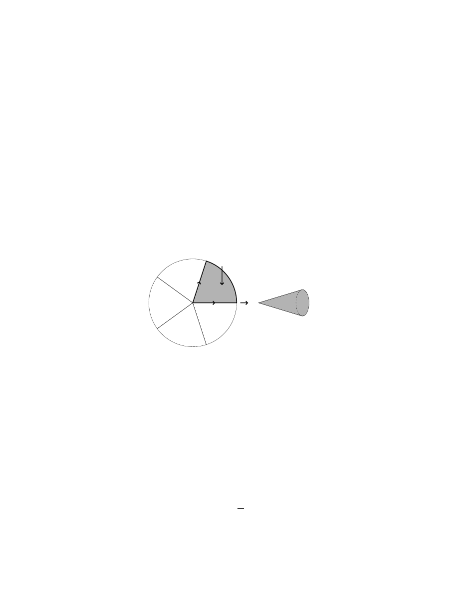
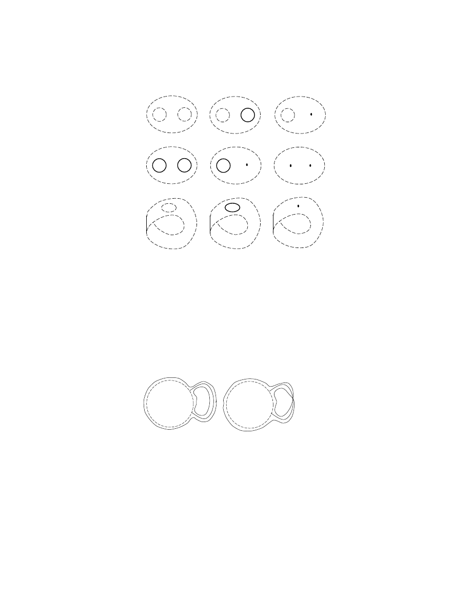
3. Orbifolds
An n-orbifold is a space that looks locally like R
n
/G where G is a finite subgroup
of GL(n, R). Note that G varies from point to point, for example, a neighborhood
of [x] ∈ R
n
/G looks like R
n
/G
x
where G
x
= {g ∈ G | gx = x}.
We will restrict, for simplicity, to locally orientable 2-orbifolds (i.e., the above
G preserves orientation). Then the only possible local structures are R
2
/C
p
, p =
1, 2, 3, . . . , where C
p
is the cyclic group of order p acting by rotations. the local
structure is then a “cone point” with “cone angle 2π/p” (Fig. 1).
fundamental domain
Figure 1
4. Some examples of geometric manifolds and orbifolds
Example 4.1. Let Λ be a group of translations of E
2
generated by two linearly
independent translations e
1
and e
2
. Then T
2
= E
2
/Λ = gives a Euclidean structure
on T
2
. We picture a fundamental domain and how the sides of the fundamental
domain are identified in Fig. 2.
Note that different choices of {e
1
, e
2
} will give different Euclidean structures
on T
2
.
Example 4.2. A classical example is the subgroup PSL(2, Z) ⊂ PSL(2, R) =
Isom
+
(H
2
), which acts on H
2
with fundamental domain pictured in Fig. 3. The
picture also shows how PSL(2, Z) identifies edges of this fundamental domain. thus
the quotient H
2
/ PSL(2, Z) is an orbifold with a 2π/2-cone-point at P , a 2π/3-cone-
point at Q, and a “cusp” at infinity (Fig. 4). It has finite 2-volume (area) as you
can check by integrating the volume form
1
y
2
dxdy over the fundamental domain:
vol(H
2
/ PSL(2, Z)) = 2π/6. We give a different proof of this in the next section.
6
1. GEOMETRIC STRUCTURES
e2
e1
Figure 2
1
0
−1
P
Q
Figure 3
P
Q
Figure 4
5. VOLUME AND EULER CHARACTERISTIC
7
5. Volume and euler characteristic
Denote by F
g
the compact orientable surface of genus g (Fig. 5 shows g = 4).
Suppose it has a geometric structure with (constant) curvature K.
Figure 5
Subdivide F
g
into many small geodesic triangles
∆
i
,
i = 1, 2, . . . , T .
Let the number of vertices of this triangulation be V , number of edges E. It is
known (Euler theorem) that
(1)
T − E + V = 2 − 2g .
By 1.1, K vol(∆
i
) = α
i
+ β
i
+ γ
i
− π, where α
i
, β
i
, γ
i
are the angles of ∆
i
, so
(2)
K vol(F
g
) =
T
X
i=1
(α
i
+ β
i
+ γ
i
− π) =
T
X
i=1
(α
i
+ β
i
+ γ
i
) − πT
= 2πV − πT
since we are summing all angles in the triangulation and around any vertex they
sum to 2π. Now 3T = 2E (a triangle has 3 edges, each of which is on two triangles),
so
(3)
T = 2E − 2T
(2) and (3) imply K vol(F
g
) = 2πV − 2πE + 2πT . By (1) this gives: K vol(F
g
) =
2π(2 − 2g).
Now suppose that instead of F
g
we have the surface of genus g with s orbifold
points with cone angles 2π/p
1
, . . . , 2π/p
s
. Then in step (2) above we must replace
s summands 2π by 2π/p
1
, . . . , 2π/p
s
, so we get instead:
K vol(F ) = 2π
Ã
2 − 2g −
s
X
i=1
µ
1 −
1
p
i
¶!
.
If we also have h cusps we must correct further by subtracting 2πh. Thus:
Theorem 5.1. If the surface F of genus g with h cusps and s orbifold points
of cone-angles 2π/p
1
, . . . , 2π/p
s
has a geometric structure with constant curvature
K then
K vol(F ) = 2πχ(F )
with
χ(F ) = 2 − 2g − h −
s
X
i=1
µ
1 −
1
p
i
.
In particular, the geometry is S
2
, E
2
, or H
2
according as χ(F ) > 0, χ(F ) = 0,
χ(F ) < 0.
¤
8
1. GEOMETRIC STRUCTURES
There is a converse (which we will not prove here, but it is not too hard):
Theorem 5.2 (Geometrization Theorem for Orbifolds). Let F be the orbifold
of Theorem 5.1. Then F has a geometric structure unless F is in the following list:
1. g = 0, h = 0, and either s = 1 or s = 2 and p
1
6= p
2
;
2. g = 0, h = 1 or 2, s = 0;
3. g = 0, h = 1, s = 1;
4. g = 0, h = 1, s = 2, p
1
= p
2
= 2.
That is: F ∼
= X/Γ where X = S
2
, E
2
, or H
2
, and Γ ⊂ Isom
+
(X) is a discrete
subgroup acting so X/Γ has finite volume. (In each of cases 2–4 the orbifold does
have an infinite-volume Euclidean structure, which is unique up to similarity. The
orbifolds of case 1 are “bad orbifolds,” that is, orbifolds which have no covering by
a manifold at all—see Sect. 14)
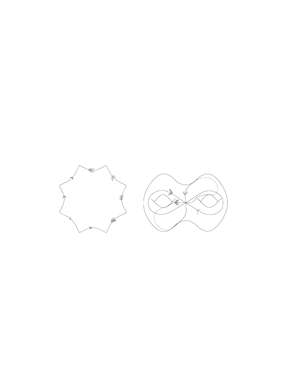
Exercise 1. Here is a hyperbolic structure on F
2
. Start with a regular octagon
in H
2
with angles 2π/8. Why does it exist? (Hint: work in the Poincar´e disk model
instead of upper half plane and expand a regular octahedron centered at the origin
from very small to very large.) Identify edges as shown in Fig. 6.
Figure 6
Note that we don’t really need a regular octahedron for this construction. All
we need is:
(i) sum of all eight angles is 2π.
(ii) pairs of edges to be identified have equal length.
It is not hard to see that this gives 8 degrees of freedom for choosing the polygon.
This gives 6 degrees of freedom for the geometric structure on F
2
since the choice
of the point P in F
2
uses 2 degrees of freedom.
In general,
Theorem 5.3. The set of geometric structures on the orbifold of Theorem 5.1
(up to isometry) is a space of dimension max{0, 6g −6+2s+2h}. It is the so-called
Teichm¨
uller moduli space of geometric structures on the orbifold. (In the E
2
case,
we must take structures up to similarity instead of isometry.)
7. A DIGRESSION: CLASSIFYING FINITE SUBGROUPS OF SO(3)
9
6. Moduli space of geometric structures on the torus
We consider two Euclidean tori equivalent if they are similar, i.e., they are
isometric after possibly uniformly scaling the metric on one of them.
See Example 4.1. A Euclidean torus is T
2
= E
2
/Λ. Choose a basis e
1
, e
2
of
Λ. By a similarity (scaling) we can assume e
1
has length 1. By a rotation we can
make e
1
= (1, 0). If we choose {e
1
, e
2
} as an oriented basis, e
2
is now in the upper
half plane. We identify R
2
= C and consider e
2
as a complex number τ . This τ is
called the complex parameter of the torus T
2
with respect to the chosen basis e
1
,
e
2
.
If we fix this basis, then τ determines the Euclidean structure on T
2
up to
similarities of T
2
which are isotopic to id
T
2
. The space of geometric structures on
an orbifold up to equivalences isotopic to the identity is called Teichm¨uller space.
Thus Teichm¨
uller space for T
2
is the upper half plane H
2
.
If we change the basis e
1
, e
2
to
e
0
2
= ae
2
+ be
1
e
0
1
= ce
2
+ de
1
with ad − bc = 1 (so it is an invertible orientation-preserving change of basis) then
τ gets changed to
τ
0
= aτ +
b
c
τ + d .
This is the action of PSL(2, Z) on H
2
. Thus:
Theorem 6.1. The (Teichm¨uller) moduli space of geometric structures on T
2
is H
2
/ PSL(2, Z). (cf. Example 3.2).
¤
7. A digression: classifying finite subgroups of SO(3)
Let G ⊂ SO(3) = Isom
+
(S
2
) be a finite subgroup. Then F = S
2
/G is an
orbifold with spherical geometric structure, so by Theorem 5.1, F satisfies 2 − 2g −
h−
s
P
i=1
³
1 −
1
p
i
´
> 0. Now h = 0 since S
2
/G is compact, and 2−2g−
P ³
1 −
1
p
i
´
> 0
clearly implies g = 0, so we get
2 −
s
X
i=1
µ
1 −
1
p
i
> 0 .
It is easy to enumerate the solutions:
|G|
s = 0
G = {1}
1
s = 1 Not allowed (“bad”—see Theorem 5.2
s = 2 p
1
= p
2
= p (p
1
6= p
2
is “bad”)
G = C
p
p
s = 3 (p
1
, p
2
, p
3
) = (2, 2, p)
G = D
2p
2p
= (2, 3, 3)
G = T
12
= (2, 3, 4)
G = O
24
= (2, 3, 5)
G = I
60
Here T , O, I are the “tetrahedral group”, “octahedral group”, “icosahedral group”
(group of orientation preserving symmetries of the tetrahedron, octahedron, and
icosahedron respectively).
10
1. GEOMETRIC STRUCTURES
We can compute the size of G from theorem 5.1:
|G| = vol(S
2
)/ vol(F ) = 4π/
µ
2π
·
2 −
X µ
1 −
1
p
i
¶¸
.
Note that G = π
1
(F ). With Theorem 14.3 this gives the standard presentation of
the above finite G ⊂ SO(3).
8. Dimension 3. The geometrization conjecture
We have seen that in dimension 2 essentially “all” orbifolds have geometric
structures. Until 1976, the idea that anything similar might hold for dimension 3
was so absurd as to be unthinkable. In 1976 Thurston formulated his
Conjecture 8.1 (Geometrization Conjecture). Every 3-manifold has a “nat-
ural decomposition” into geometric pieces.
The decomposition in question had already been proved in a topological version
by Jaco & Shalen and Johannson, as we describe in Chapter 2. One may assume by
earlier results of Knebusch and Milnor (cf. [27]) that M
3
is connected-sum-prime,
and M
3
then has a natural “JSJ decomposition” (also called “toral decomposition”)
which cuts M
3
along embedded tori
1
into pieces which are one of
1. Seifert fibered with circle fibers (Seifert fibered means fibered over an
orbifold, see Chapter 2);
2. not Seifert fibered with circle fibers but Sefert fibered over a 1-orbifold
(i.e., S
1
or I) with T
2
-fibers (in the I case there are special fibers—Klein
bottles—over the endpoints of I);
3. simple (see below), but not Seifert fibered.
We will discuss the geometrization conjecture for these three cases after defining
“simple.” We are interested in a manifold M
3
that is the interior of a compact
manifold-with-boundary M
3
such that ∂M
3
is a (possibly empty) union of tori
(briefly “M
3
has toral ends”). This is because M
3
may have resulted via the JSJ
decomposition theorem by cutting a compact manifold along tori.
Definition 8.2. M
3
is simple if every essential embedded torus (that is, one
that doesn’t bound a solid torus in M
3
) is isotopic to a boundary component of M .
The geometrization conjecture is true (and easy) in cases 1 and 2 above. In
case 3 it splits into two conjectures:
Conjecture 8.3. A 3-manifold with |π
1
(M
3
)| < ∞ is homeomorphic to S
3
/G
for some finite subgroup G ⊂ Isom
+
(S
3
).
Conjecture 8.4. A simple 3-manifold with |π
1
(M
3
)| = ∞ which is not Seifert
fibered has a hyperbolic structure.
Conjecture 8.3 is equivalent to the combination of two old and famous unsolved
conjectures:
Conjecture 8.5 (Poincar´e Conjecture). π
1
(M
3
) = {1} ⇒ M
3
∼
= S
3
.
Conjecture 8.6 (Space-Form-Conjecture). A free action of a finite group on
S
3
is equivalent to a linear action.
1
The geometric version of the decomposition uses both tori and Klein bottles, see Sect. 6 of
Chapter 2.
10. THE HYPERBOLIC GEOMETRIZATION CONJECTURE
11
9. Geometrization in the “easy” cases
There are 8 geometries relevant to 3-manifolds. They are called S
3
, Nil, PSL,
Sol, H
3
, S
3
× E
1
, E
3
, H
2
× E
1
.
A Seifert fibered manifold with circle fibers is fibered M
3
→ F
2
over an orbifold
F
2
of dimension 2. If M
3
is closed there are two invariants associated with this
situation:
• The orbifold euler characteristic χ(F
2
) (see Section 3 of this chapter).
• The euler number of the Seifert fibration e(M
3
→ F
2
) (see Section 4 of
Chapter 2).
and the relevant geometry is determined by these as:
χ > 0
χ = 0
χ < 0
e 6= 0
S
3
Nil
PSL
e = 0 S
2
× E
1
E
3
H
2
× E
1
If the Seifert fibered manifold M
3
is not closed then e(M
3
→ F
2
) is not well
defined (it depends on a choice of “slopes” on the toral ends of M
3
) so M
3
can
have either a PSL or a H
2
× E
1
structure. There are three exceptional cases:
D
2
× S
1
, T
2
× (0, 1) and a manifold 2-fold covered by the latter (interval bundle
over Klein bottle) each have infinite volume complete E
3
structures but no finite
volume geometric structure.
For more details on the above see [30] or [41].
Case 2 of the “easy cases” is manifolds with Sol-structures. Only closed mani-
folds occur for this geometry.
This leaves only H
3
to discuss.
10. The hyperbolic geometrization conjecture
There are several models for H
3
. One of the often used ones is the upper half
space model:
{(z, r) ∈ C × R | r > 0} with metric ds =
p
dx
2
+ dy
2
+ dr
2
/r,
where z = x + iy. The orientation preserving isometry group is Isom
+
(H
3
) =
PSL(2, C).
Recall Conjecture 8.4:
Conjecture. If M is simple and not Seifert fibered and |π
1
(M )| = ∞ then
M has a hyperbolic structure.
This had been proved by Thurston in the following situations
• M
3
is Haken (see Chapter 2 for the definition; this is true if for instance
if |H
1
(M )| = ∞)
• M has a finite symmetry with positive dimensional fixed point set,
but not all details of the second case are published yet (see [46], [29], [8]). This
conjecture and the special cases proven so far have had a major effect on 3-manifold
theory, including helping toward the solutions of several old conjectures, e.g., the
Smith Conjecture ([29]) and various conjectures about knots.
12
1. GEOMETRIC STRUCTURES
11. Examples of a hyperbolic 3-manifold and orbifolds
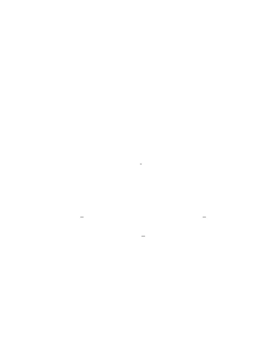
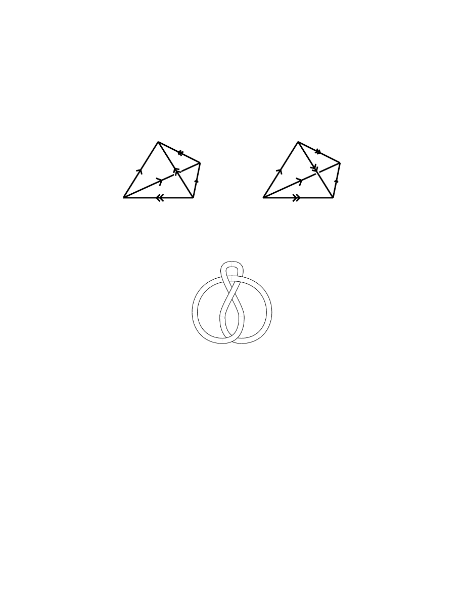
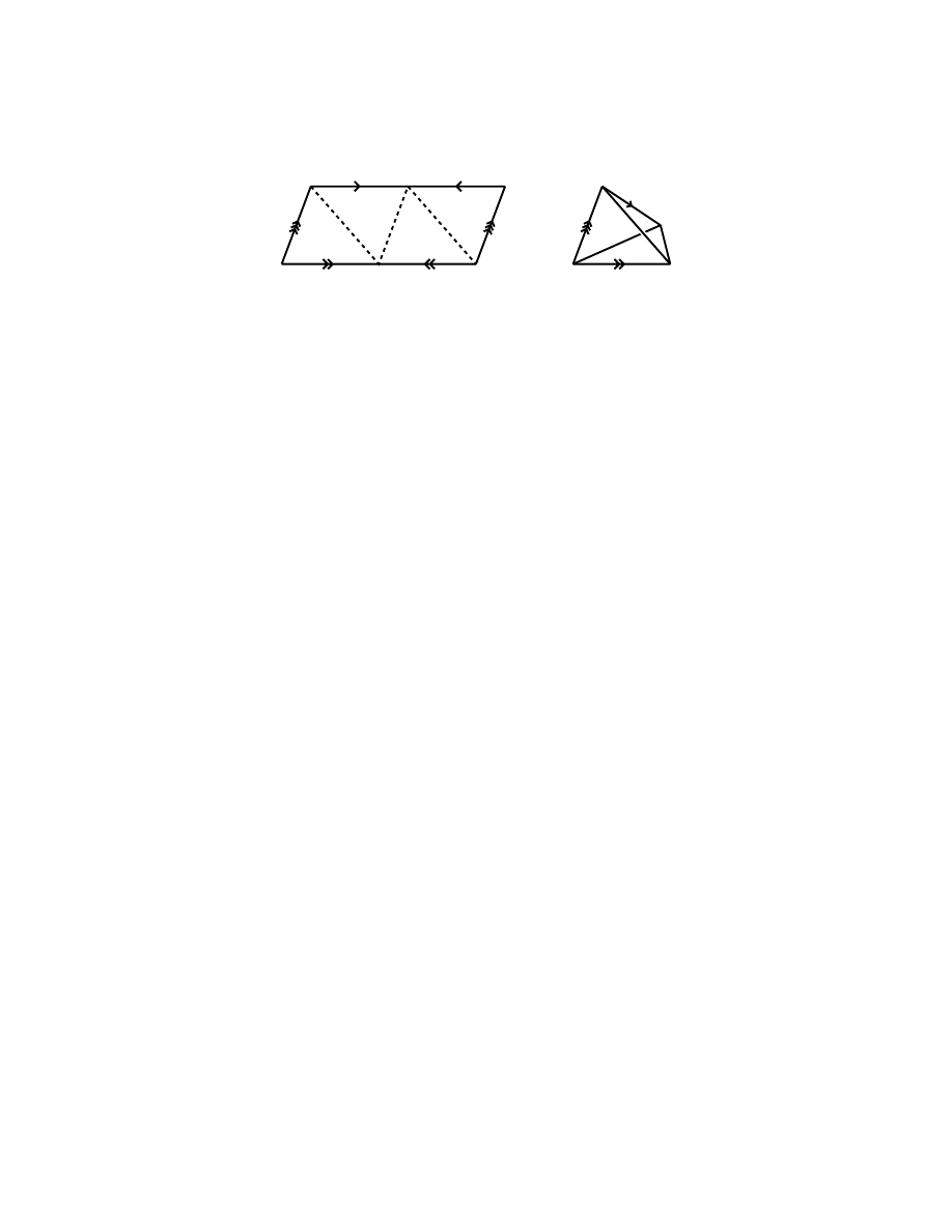
Example 11.1. Take two regular ideal tetrahedra in H
3
(i.e., vertices are “at
infinity”). Paste pairs of faces together as directed by Fig. 7, so correspondingly
marked edges match up (there is just one way to do this).
Figure 7
The result is a hyperbolic structure on the complement in S
3
of the figure-8
knot, pictured in Fig. 8
Figure 8
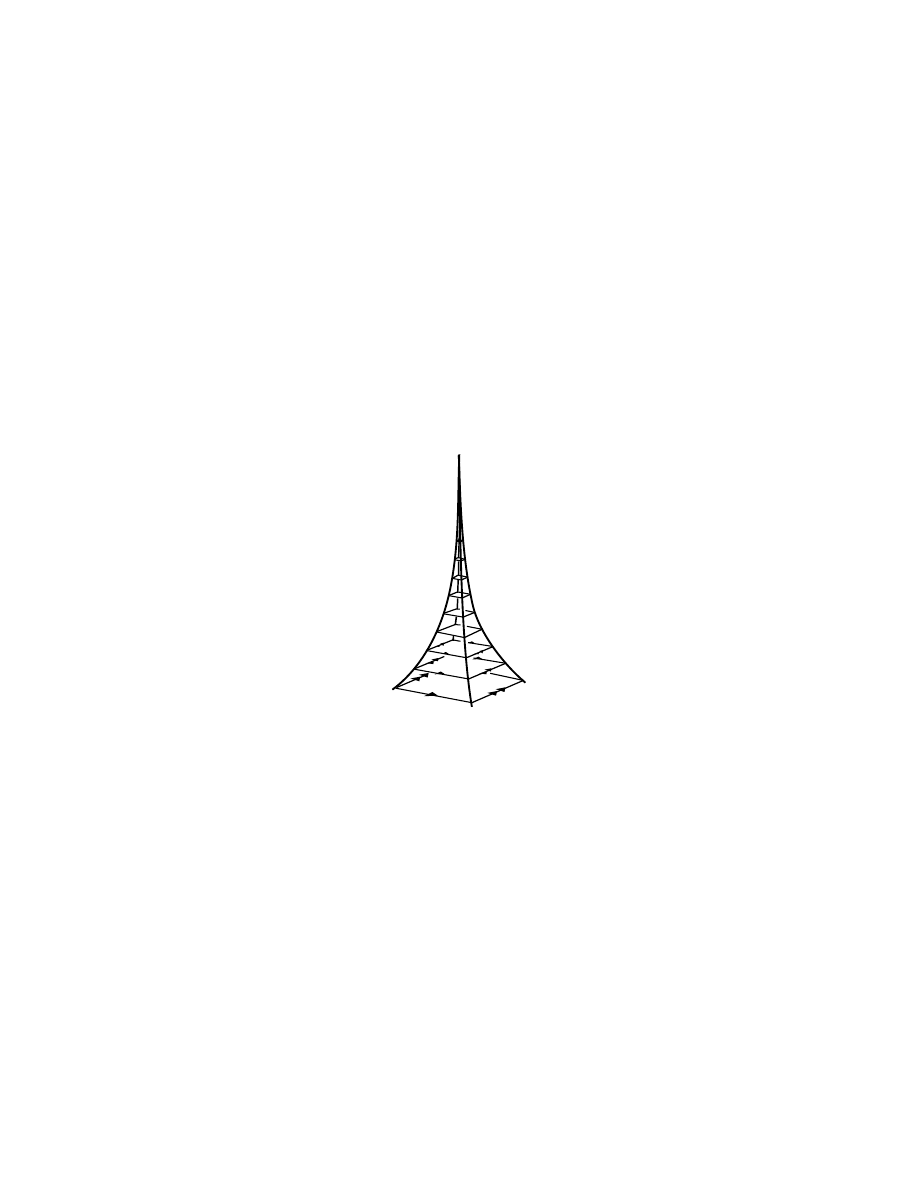
Example 11.2. Consider the tesselation of H
3
by copies of the regular ideal
tetrahedron (I can’t draw this, so Fig. 9 shows the analogous picture for dimension
n = 2). Call this tetrahedral tesselation τ
0
.
Let Γ
0
⊂ PSL(2, C) be the group of all symmetries (preserving orientation) of
this tesselation.
• Q
0
= H
3
/Γ
0
is the smallest orientable orbifold with a cusp (Meyerhoff
[26]).
• Q
0
is 24-fold covered by the Figure-8 knot complement.
• Q
0
= H
3
/P GL(2, O
3
), so it is arithmetic (see Chapter 3 for the definition).
Example 11.3. τ
1
= tesselation of H
3
by regular ideal octahedra. Γ
1
= group
of orientation preserving symmetries of τ
1
. Q
1
= H
3
/Γ
1
.
• Q
1
is the second smallest orientable cusped orbifold (Adams [2]).
• Q
1
= PGL(2, O
1
).
• Q
1
has a double cover which is the orbifold whose volume is the smallest
“limit volume” (see Sect. 16) (Adams [1]).
• Q
1
is 24-fold covered by the Whitehead link complement.
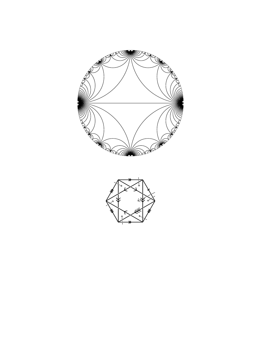
12. RIGIDITY IN DIMENSION 2: TRIANGLE ORBIFOLDS
13
Figure 9
B´
A´
C´
C
B
D´
D
A
Figure 10
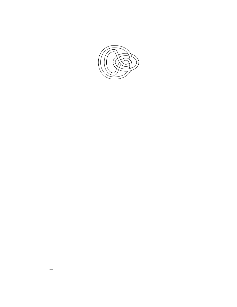
Example 11.4. Consider a regular ideal octahedron with faces identified as in
Fig. 10 (match A to A
0
, B to B
0
, etc.)
Result: Complement of the Whitehead link (Fig. 11).
12. Rigidity in dimension 2: triangle orbifolds
A triangle orbifold is a 2-dimensional orbifold with g = 0, s + h = 3. A triangle
orbifold is obtained by gluing together two copies of a triangle of the appropriate
geometry (this triangle has ideal vertices if h > 0). We speak of the (p
1
, p
2
, p
3
)-
triangle if the angles of the triangle are π/p
1
, π/p
2
, π/p
3
with p
i
∈ {2, 3, 4, . . . , ∞}.
For example H
2
/ PSL(2, Z) is the (2, 3, ∞)-triangle orbifold.
14
1. GEOMETRIC STRUCTURES
Figure 11
A triangle orbifold has unique geometric structure, as does the orbifold S
2
/C
p
with g = 0, h = 0, s = 2. In all other cases the dimension 6g − 6 + 2s + 2h of
Teichm¨
uller space is positive, so there are infinitely many geometric structures.
Dimension 3 is in sharp contrast to this:
13. Mostow-Prasad rigidity
Theorem 13.1 (Mostow-Prasad). The hyperbolic structure on a hyperbolic 3-
orbifold is unique. In fact (stronger formulation): If Γ
1
and Γ
2
are discrete sub-
groups of PSL(2, C) = Isom
+
(H
3
) such that
(i) H
3
/Γ
1
is a finite volume orbifold, and
(ii) Γ
1
∼
= Γ
2
,
then any isomorphism Γ
1
→ Γ
2
is induced by an inner automorphism (conjugation)
in PSL(2, C). In particular, H
3
/Γ
1
∼
= H
3
/Γ
2
(isometry).
This is a remarkable result. The geometrization conjecture says that “almost
every” 3-manifold has a hyperbolic structure, and rigidity says this structure is
unique! Thus any information we extract from the geometry is actually a topological
invariant of the manifold. Usually it is hard to find topological descriptions of the
resulting invariants, but there is an elegant topological invariant of a 3-manifold
called “Gromov norm” (after its inventor) which equals a constant multiple of the
volume for a hyperbolic 3-manifold.
In later lectures we will describe arithmetic invariants of the hyperbolic struc-
ture. Again, by rigidity, these invariants are topological invariants.
14. Fundamental Group and Covering Spaces
We have referred to fundamental groups and covering spaces of orbifolds above.
For our purposes we can define the fundamental group of an orbifold similarly to
the standard definition for spaces (our definition depends on the fact that we only
consider orientable orbifolds—the codimension 1 sets of orbifold points that occur
in non-orientable ones need extra technicalities):
Let F be an orientable orbifold, ∗ ∈ F a base-point. π
1
(F ) = set of “homotopy
classes” of closed paths γ : [0, 1] → F , γ{0, 1} = {∗} which do not pass through
any orbifold points. “Homotopy” now means deformation of paths in which the
deformation may pass through orbifold points, but when it does, the deformation
in the “local picture” U/G must be the image of a deformation in U , cf. Fig. 12 (a
2π
2
-cone-point).
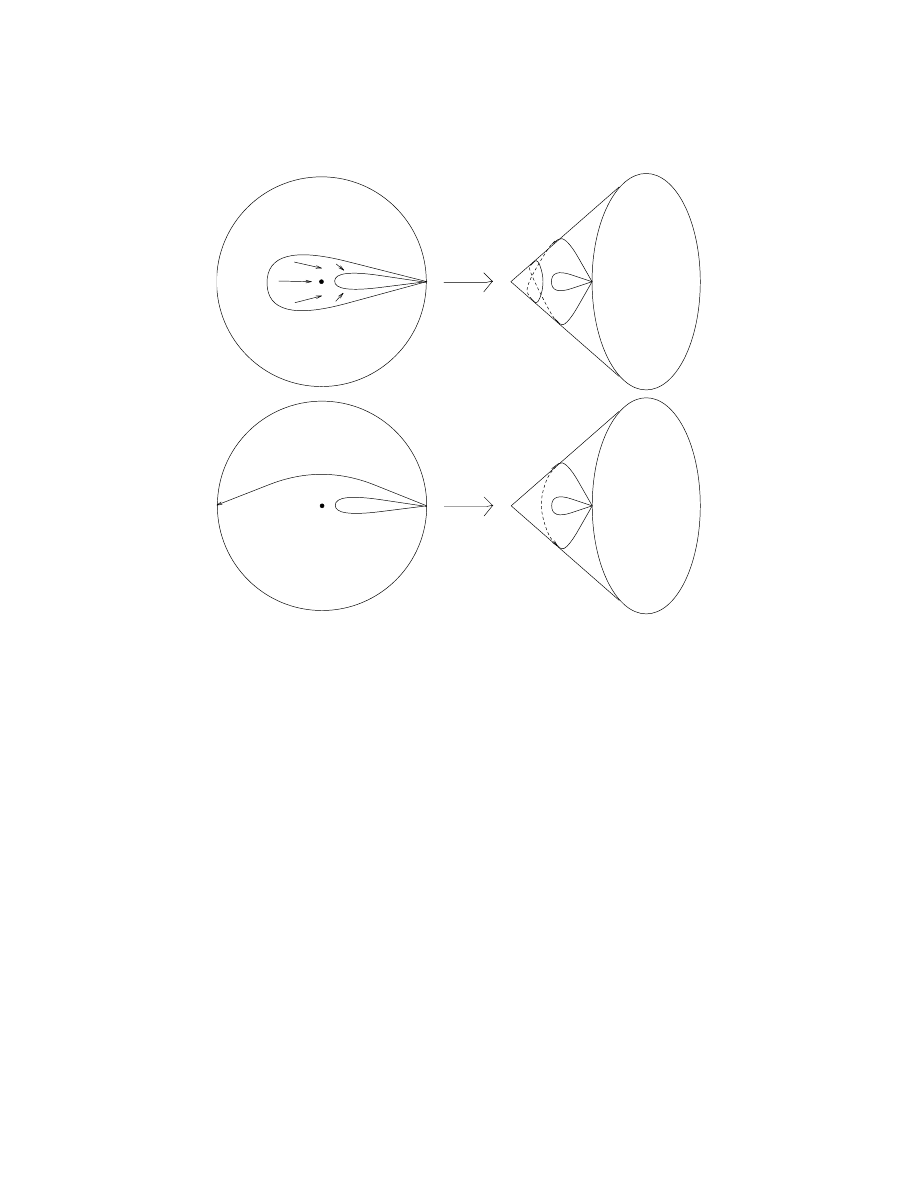
14. FUNDAMENTAL GROUP AND COVERING SPACES
15
2
U/C
U
allowed deformation
2
U/C
U
not allowed
Figure 12
14.1. Covering Spaces. Recall that, for us, orbifolds arose as orbit spaces
X/Γ of properly discontinuous group actions on manifolds (or other orbifolds).
From this point of view it is easy to define coverings.
Definition 14.1. f : M → N is a covering map of orbifolds if one can express
M and N , as orbifolds, as X/Λ and X/Γ, for some X, so that Λ ⊂ Γ and f : M → N
is the natural map X/Λ → X/Γ.
Theorem 14.2. (Connection between π
1
(F ) and coverings) Let F be a con-
nected oriented orbifold, Γ = π
1
(F ). then there exists an orbifold e
F with a properly
discontinuous action of Γ such that F = e
F /Γ. Any covering M → F with M
connected has the form e
F /Λ → F = e
F /Γ for some group Λ ⊂ Γ.
e
F → F is called the universal covering of F . If e
F is a manifold then F is called
a good orbifold.
Theorem 14.2 is proved for spaces in many text-books on topology. It is a good
exercise to take such a proof and re-write it for orbifolds. It is also a good exercise
to take the computation of the fundamental group of a surface, that can be found
in many textbooks, and generalize it to show:
16
1. GEOMETRIC STRUCTURES
Theorem 14.3. The orbifold F (g; h; p
1
, . . . , p
s
) of genus g with h punctures
and s orbifold points of the types p
1
, . . . , p
s
has
π
1
(F (g; h; p
1
, . . . , p
s
)) =ha
1
, . . . , a
g
, b
1
, . . . , b
g
, q
1
, . . . q
s+h
|
q
p
1
1
= 1, . . . , q
p
s
s
= 1, q
1
. . . q
s+h
[a
1
, b
1
] . . . [a
g
, b
g
] = 1i
.
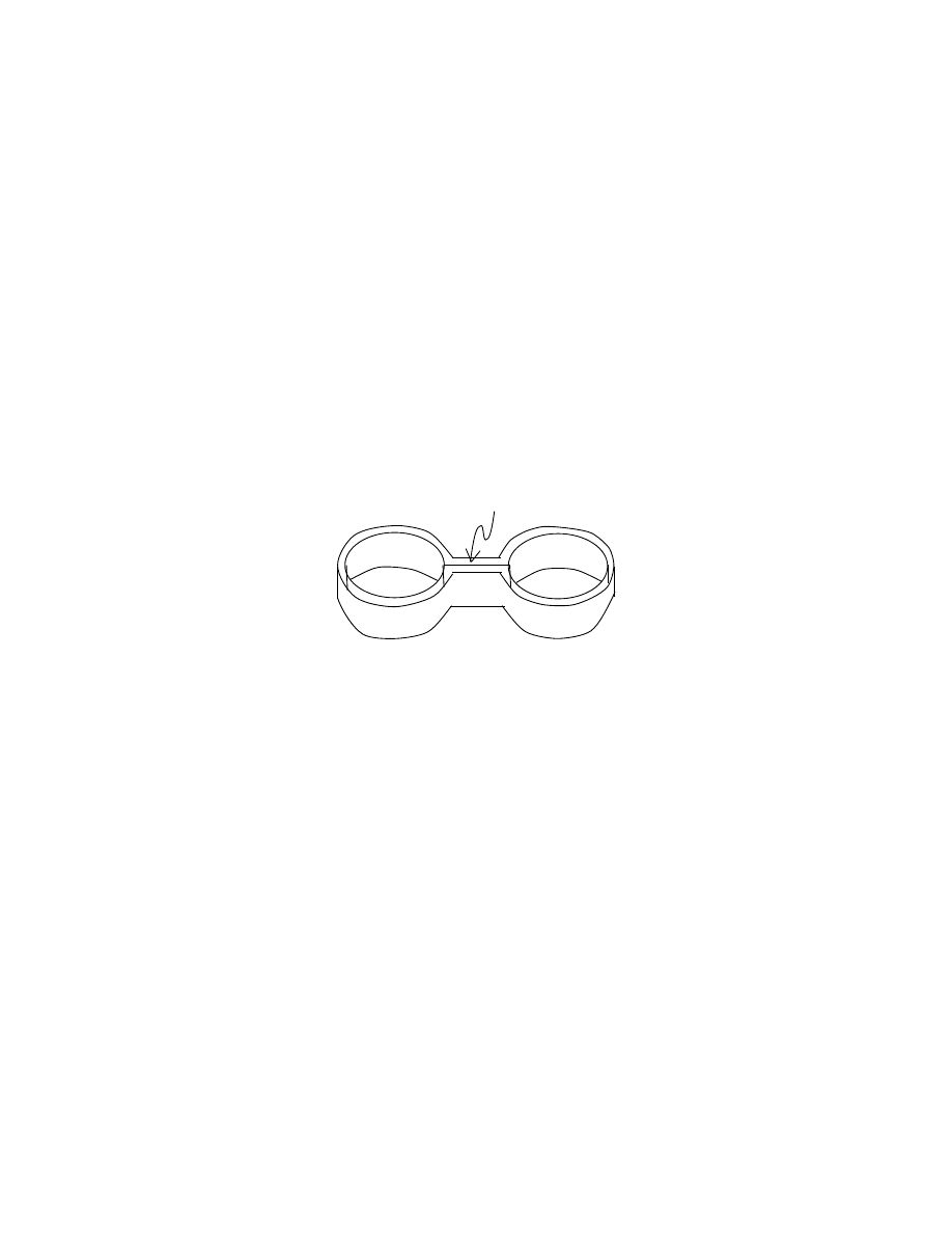
15. Cusps of hyperbolic 3-orbifolds
Where a hyperbolic 3-manifold is non-compact, the local structures is that of
a cusp
C = {(x + iy, r) | r > K}/Λ
where Λ is a lattice of horizontal translations. Horizontal cross-sections (r = con-
stant) of C are Euclidean tori which are shrinking in size as r → ∞.
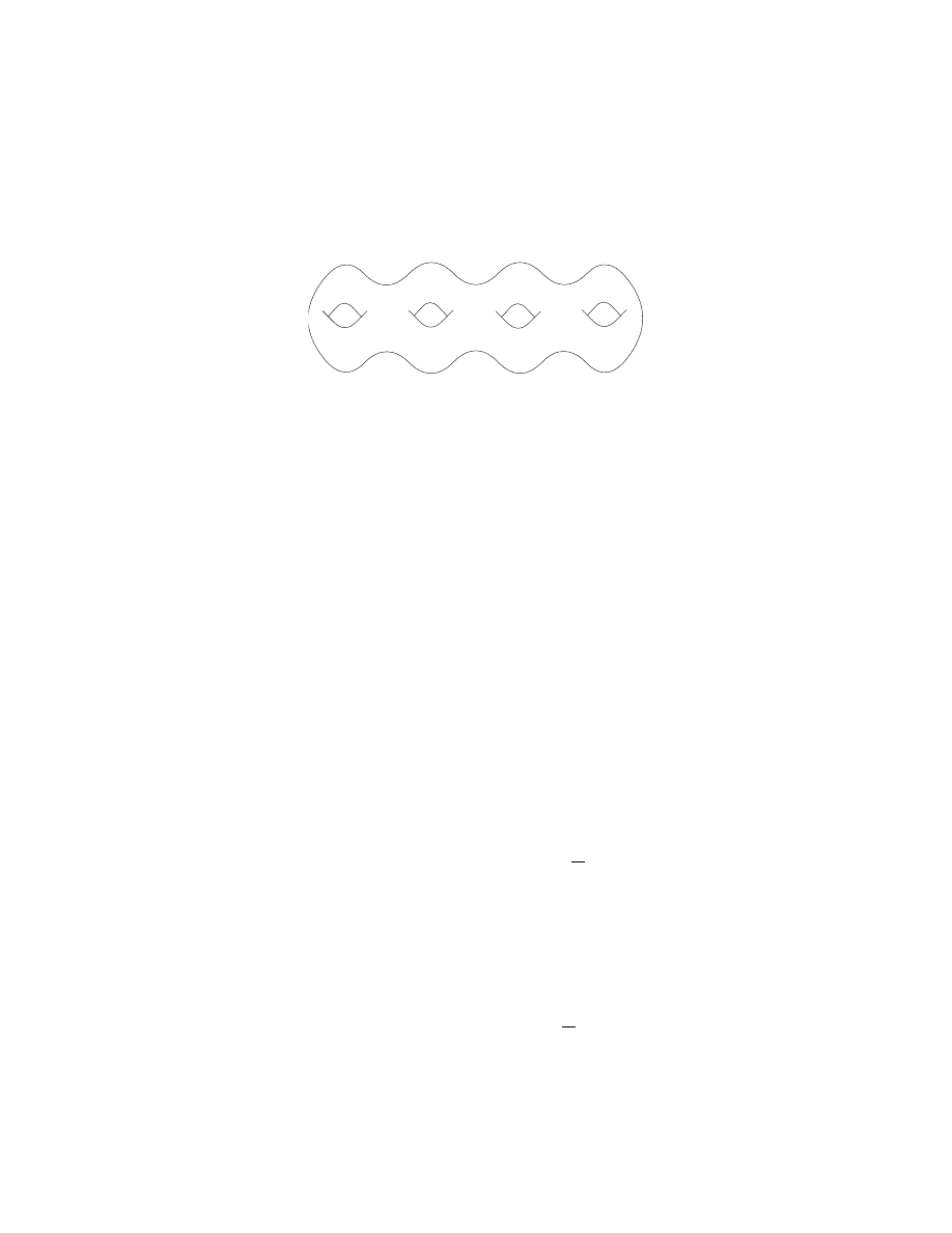
Figure 13
The (r = constant) cross-sections of C are called horosphere sections.
In a hyperbolic 3-orbifold the picture is the same except that the horosphere
sections of a cusp can be any Euclidean orbifold. The Euclidean orbifolds are easily
classified.
Exercise 2. Do this analogously to Section 7—solve the equation χ = 0 to
show they are
• the Euclidean tori E
2
/Λ;
• the triangle orbifolds (cf. Section 12) with (p
1
, p
2
, p
3
) = (2, 4, 4), (2, 3, 6),
or (3, 3, 3);
• orbifolds with g = 0, h = 0, s = 4, and (p
1
, p
2
, p
3
, p
4
) = (2, 2, 2, 2). We
call these “pillow orbifolds.”
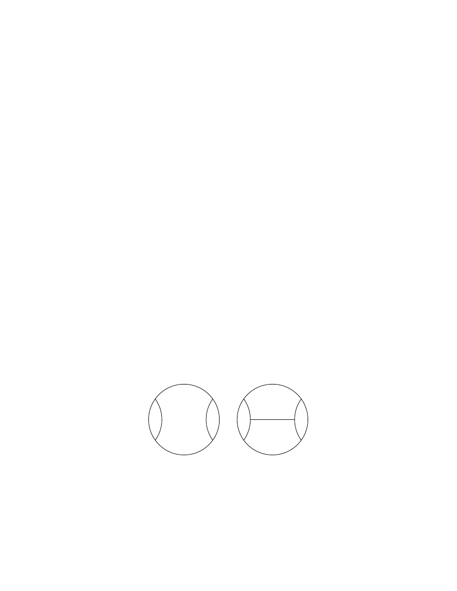
Exercise 3. Fig. 14 shows a pillow orbifold with an embedding of it as a the
surface of a tetrahedron in E
3
. Show that if one allows degenerate (flat) tetra-
hedra, every pillow orbifold has a unique embedding as the surface of a euclidean
tetrahedron up to isometry.
16. VOLUMES OF HYPERBOLIC ORBIFOLDS
17
Figure 14
The Euclidean triangle orbifolds are rigid (see Section 12) but the Euclidean
tori and pillow orbifolds have 2-dimensional spaces of deformations of the Euclidean
structure. In fact, every Euclidean torus double covers a unique Euclidean pillow
orbifold and vice versa (the torus E
2
/Λ double covers E
2
/Γ, where Γ ⊂ Isom
+
(E
2
) is
generated by Λ and the map
¡
−1 0
0 −1
¢
: E
2
→ E
2
), so the Teichm¨
uller moduli space
of pillow orbifolds is the same as for tori, namely H
2
/ PSL(2, Z)—see Theorem 6.1
Definition 15.1. If a cusp of a hyperbolic 3-orbifold has horosphere sections
which are tori or pillow orbifolds the cusp is called non-rigid, if the horosphere
sections are triangle orbifolds the cusp is rigid.
The non-rigid cusps are important for “hyperbolic Dehn surgery,” as we shall
describe later. One effect of this is that they affect the volume of the orbifold in a
way that we can already describe.
16. Volumes of hyperbolic orbifolds
Theorem 16.1. (Thurston, Jørgenson) The set Vol = {v ∈ R | v is the volume
of some hyperbolic 3-orbifold} is a well ordered closed subset of R of order type ω
ω
.
To each v ∈ Vol there are just finitely many orbifolds of this volume.
Otherwise expressed: the elements of Vol are ordered
v
0
< v
1
< v
2
< · · · < v
ω
< v
ω+1
< · · · < v
2ω
< · · · < v
3ω
< · · ·
· · · < v
ω
2
< · · · < v
κ
< · · · .
The general index κ is an infinite ordinal number
κ = a
n
ω
n
+ a
n−1
ω
n−1
+ · · · + a
0
and a
i
∈ {0, 1, 2, . . . }
If κ is divisible by ω then v
κ
is the limit of the v
λ
, λ < κ; we say v
κ
is a limit
volume. If κ is divisible by ω
2
then v
κ
is a limit of limit volumes—it is a 2-fold
limit volume. If κ is divisible by ω
n
then v
κ
is an n-fold limit volume (limit of
(n − 1)-fold limit volumes).
Theorem 16.2. If M is a hyperbolic orbifold with n non-rigid cusps, then
vol(M ) is an n-fold limit volume.
A few of the v
κ
are known: Colin Adams has found v
ω
, v
2ω
, and v
3ω
. He
has also found the six non-compact orbifolds of least volume (with rigid cusps; the
smallest of these has been earlier found by Meyerhoff). See [1] and [2].
No-one knows v
0
(although there is a guess, namely 0.03905 . . ., known to be the
smallest volume in the arithmetic case, [6]). The smallest hyperbolic manifold is
even harder to determine, but again there is a guess, with volume about .942707 . . .,
again known to be smallest among arithmetic hyperbolic 3-manifolds [7].
The minimal examples found so far are all arithmetic (see Chapter 3 or [33]
for a definition). This is striking, because arithmetic examples are very sparse
18
1. GEOMETRIC STRUCTURES
overall—Borel showed in [5] that there are only finitely many with volume below
any given bound.
17. Hyperbolic Dehn surgery
Let M be a hyperbolic orbifold with a cusp C whose horosphere section (cf.
Section 15) is a torus. If we cut off the cusp C, we obtain a manifold M
0
with
boundary: ∂M
0
= T
2
.
If we write T
2
= E
2
/Λ and choose a basis e
1
, e
2
for Λ, then for any coprime
pair of integers (p, q), the element pe
1
+ qe
2
determines a simple curve on T
2
.
We can glue a solid torus D
2
× S
1
to M
0
along the boundary T
2
in such
a way that the curve pe
1
+ qe
2
in ∂M
0
matches up with the “meridian curve”
∂D
2
× {1} ⊂ ∂(D
2
× S
1
). The result of this pasting will be called M (p, q):
M (p, q) = M
0
[
T
2
D
2
× S
1
such that pe
1
+ qe
2
= ∂D
2
× {1} .
If p and q are not coprime we define M (p, q) as an orbifold as follows. Let d =
gcd(p, q), p
0
= p/d, q
0
= q/d. The underlying space of M (p, q) is M (p
0
, q
0
) but we
put a cone-angle of 2π/d transverse to the core circle of D
2
× S
1
. That is, instead
of D
2
× S
1
we use the orbifold (D
2
/C
d
) × S
1
.
Terminology M (p, q) is a (p, q)-Dehn-filling of M .
Theorem 17.1. (Thurstons’ Dehn Surgery Theorem) For all but at most finitely
many (p, q) ∈ Z×Z−{(0, 0)}, the orbifold M (p, q) has a hyperbolic structure. More-
over
vol(M (p, q)) < vol(M )
and
lim
(p,q)→∞
vol(M (p, q)) = vol(M ) .
If M has a pillow cusp (see Section 15), then one can still define (p, q)-Dehn
filling. Remember that the pillow orbifold is T
2
/C
2
where C
2
acts on T
2
= E
2
/Λ
by the matrix
¡
−1 0
0 −1
¢
. This action of C
2
extends to the solid torus D
2
× S
1
, so
instead of pasting in D
2
×S
1
, one pastes in the orbifold (D
2
×S
1
)/C
2
. This orbifold
is a 3-disk with two curves through it with transverse cone angle 2π/2, cf. Fig. 15a.
If gcd(p, q) = d, there are additional orbifold points; cf. Fig. 15b.
2
2
(a)
d
2
2
(b)
Figure 15
The Dehn surgery theorem explains how a non-rigid cusp of M makes vol(M )
a limit volume (so n non-rigid cusps makes vol(M ) an n-fold limits volume).
Theorem 16.1 follows from the Dehn surgery theorem and the following

19. NON-ORIENTABLE 2-ORBIFOLDS
19
Proposition 17.2. For any bound V there is a finite collection of hyperbolic
orbifolds such that every hyperbolic orbifold with volume ≤ V results from Dehn
surgery on a member of the collection.
18. Postscript
If one believes the geometrization conjecture, and most topologists do, then
understanding hyperbolic 3-manifolds is by far the biggest part of understanding
all 3-manifolds. Many general topological questions remain unsolved for hyperbolic
manifolds, for instance, does every hyperbolic manifold have a finite covering space
with infinite homology, or which even fibers over S
1
(Thurston’s question)? This
is not even known for the much more restricted class of arithmetic hyperbolic 3-
manifolds.
Of course, one of the most basic questions in most fields is the classification
question. Can one find a reasonable classification of hyperbolic 3-manifolds? Al-
though we are far from such a thing at present, it may not be an entirely hopeless
project in the long run—Proposition 17.2 could be a starting point. An excellent
tool for the computational study of hyperbolic 3-manifolds exists in Jeff Weeks’
computer program “snappea,” available for various computers, and the program
“snap” based on it. These have already been used to help classify non-compact hy-
perbolic manifolds that can be triangulated with few ideal simplices, for example.
19. Non-orientable 2-orbifolds
If a 3-manifold is Seifert fibred over a 2-orbifold the 2-orbifold may be non-
orientable even if the 3-manifold is orientable. The 2-orbifold will, however, be
locally orientable. We will use g < 0 for genus of non-orientable surfaces (so
g = −1, −2, . . . is projective plane, Klein bottle, ...). The euler characteristic
of the closed surface of genus g < 0 is 2 + g, so in theorem 5.1 we must replace
2 − 2g by 2 + g if g < 0. Theorem 5.2 remains true with the additional exception:
2
0
. g = 0, h = 1, s = 0.
If one drops the condition of local orientability then one also has the local
structures given by the dihedral groups of order 2n, n = 1, 2, . . . .
Exercise 4. Generalise Theorems 5.1 and 5.2 to allow non-locally-orientable
2-orbifolds and then use the method of Section 7 to classify all compact spherical
and euclidean orbifolds. This gives the classifications of all finite subgroups of
O(3) and of the so called “seventeen wallpaper groups” (a misnomer, since most
of the seventeen have positive dimensional Teichm¨uller spaces and are thus infinite
families of groups).


CHAPTER 2
Classical Theory and JSJ Decomposition
1. Dehn’s Lemma, Loop and Sphere Theorems
Theorem 1.1 (Dehn’s Lemma). If M
3
is a 3-manifold and f : D
2
→ M
3
a map
of a disk such that for some neighbourhood N of ∂D
2
the map f |N is an embedding
and f
−1
(f (N )) = N . Then f |∂D
2
extends to an embedding g : D
2
→ M
3
.
Dehn’s proof of 1910 [10] had a serious gap which was pointed out in 1927 by
Kneser. Dehn’s Lemma was finally proved by Papakyriakopoulos in 1956, along
with two other results, the loop and sphere theorems, which have been core tools
ever since. These theorems have been refined by various authors since then. The
following version of the loop theorem contains Dehn’s lemma. It is due to Stallings
[43].
Theorem 1.2 (Loop Theorem). Let F
2
be a connected submanifold of ∂M
3
, N
a normal subgroup of π
1
(F
2
) which does not contain ker(π
1
(F
2
) → π
1
(M
3
)). Then
there is a proper embedding g : (D
2
, ∂D
2
) → (M
3
, F
2
) such that [g|∂D
2
] 6∈ N .
Theorem 1.3 (Sphere Theorem). If N is a π
1
(M
3
)-invariant proper subgroup
of π
2
(M
3
) then there is an embedding S
2
→ M
3
which represents an element of
π
2
(M
3
) − N .
(These theorems also hold if M
3
is non-orientable except that in the Sphere
Theorem we must allow that the map S
2
→ M
3
may be a degree 2 covering map
onto an embedded projective plane.)
The proofs of the results in this section and the next can be found in several
books on 3-manifolds, for example [25].
2. Some Basics
Definition 2.1. An embedded 2-sphere S
2
⊂ M
3
is essential or incompressible
if it does not bound an embedded ball in M
3
. M
3
is irreducible if it contains no
essential 2-sphere.
Note that if M
3
has an essential 2-sphere that separates M
3
(i.e., M
3
falls
into two pieces if you cut along S
2
), then there is a resulting expression of M as a
connected sum M = M
1
#M
2
(to form connected sum of two manifolds, remove the
interior of a ball from each and then glue along the resulting boundary components
S
2
). If M
3
has no essential separating S
2
we say M
3
is prime
Exercise 5. M
3
prime ⇔ Either M
3
is irreducible or M
3
' S
1
× S
2
. Hint
1
.
1
Don’t read this footnote unless you want a hint. If M
3
is prime but not irreducible then
there is an essential non-separating S
2
. Consider a simple path γ that departs this S
2
from one
side in M
3
and returns on the other. Let N be a closed regular neighbourhood of S
2
∪ γ. What
is ∂N ? What is M
3
− N ?
21

22
2. JSJ DECOMPOSITION
Theorem 2.2 (Kneser and Milnor). Any 3-manifold has a unique connected
sum decomposition into prime 3-manifolds (the uniqueness is that the list of sum-
mands is unique up to order).
We next discuss embedded surfaces other than S
2
. Although we will mostly
consider closed 3-manifolds (i.e., compact without boundary), it is sometimes nec-
essary to consider manifolds with boundary. If M
3
has boundary, then there are
two kinds of embeddings of surfaces that are of interest: embedding F
2
into ∂M
3
or embedding F
2
so that ∂F
2
⊂ ∂M
3
and (F
2
− ∂F
2
) ⊂ (M
3
− ∂M
3
). The latter
is usually called a “proper embedding.” Note that ∂F
2
may be empty. In the
following we assume without saying that embeddings of surfaces are of one of these
types.
Definition 2.3. If M
3
has boundary, then a properly embedded disk D
2
⊂ M
3
is essential or incompressible if it is not “boundary-parallel” (i.e., it cannot be
isotoped to lie completely in ∂M
3
, or equivalently, there is no ball in M
3
bounded
by this disk and part of ∂M
3
). M
3
is boundary irreducible if it contains no essential
disk.
If F
2
is a connected surface 6= S
2
, D
2
, an embedding F
2
⊂ M
3
is incompress-
ible if π
1
(F
2
) → π
1
(M
3
) is injective. An embedding of a disconnected surface is
incompressible if each component is incompressibly embedded.
It is easy to see that if you slit open a 3-manifold M
3
along an incompressible
surface, then the resulting pieces of boundary are incompressible in the resulting
3-manifold. The loop theorem then implies:
Proposition 2.4. If F
2
6= S
2
, D
2
, then a two-sided embedding F
2
⊂ M
3
is
compressible (i.e., not incompressible) if and only if there is an embedding D
2
→
M
3
such that the interior of D
2
embeds in M
3
− F
2
and the boundary of D
2
maps
to an essential simple closed curve on F
2
.
(For a one-sided embedding F
2
⊂ M
3
one has a similar conclusion except that
one must allow the map of D
2
to fail to be an embedding on its boundary: ∂D
2
may map 2-1 to an essential simple closed curve on F
2
. Note that the boundary of
a regular neighbourhood of F
2
in M
3
is a two-sided incompressible surface in this
case.)
Exercise 6. Show that if M
3
is irreducible then a torus T
2
⊂ M
3
is compress-
ible if and only if either
2
• it bounds an embedded solid torus in M
3
, or
• it lies completely inside a ball of M
3
(and bounds a knot complement in
this ball).
A 3-manifold is called sufficiently large if it contains an incompressible sur-
face, and is called Haken if it is irreducible, boundary-irreducible, and sufficiently
large. Fundamental work of Haken and Waldhausen analysed Haken 3-manifolds
by repeatedly cutting along incompressible surfaces until a collection of balls was
reached (it is a theorem of Haken that this always happens). A main result is
Theorem 2.5 (Waldhausen). If M
3
and N
3
are Haken 3-manifolds and we
have an isomorphism π
1
(N
3
) → π
1
(M
3
) that “respects peripheral structure” (that
2
In the version of these notes distributed at the course the second case was omitted. I am
grateful to Patrick Popescu for pointing out the error.

3. JSJ DECOMPOSITION
23
is, it takes each subgroup represented by a boundary component of N
3
to a a conju-
gate of a subgroup represented by a boundary component of M
3
, and similarly for the
inverse homomorphism). Then this isomorphism is induced by a homeomorphism
N
3
→ M
3
which is unique up to isotopy.
The analogous theorem for surfaces is a classical result of Nielsen.
We mention one more “classical” result that is a key tool in Haken’s approach.
Definition 2.6. Two disjoint surfaces F
2
1
, F
2
2
⊂ M
3
are parallel if they bound
a subset isomorphic to F
1
× [0, 1] between them in M
3
.
Theorem 2.7 (Kneser-Haken finiteness theorem). For given M
3
there exists a
bound on the number of disjoint pairwise non-parallel incompressible surfaces that
can be embedded in M
3
.
3. JSJ Decomposition
We shall give a recent quick proof of the main “JSJ decomposition theorem”
which describes a canonical decomposition of any irreducible boundary-irreducible
3-manifold along tori and annuli.
We shall just describe it in the case that the boundary of M
3
is empty or
consists of tori. Then only tori occur in the JSJ decomposition (see section 5). An
analogous proof works in the general torus-annulus case (see [34]), but the general
case can also be deduced from the case we prove here.
The theory of such decompositions for Haken manifolds with toral boundaries
was first outlined by Waldhausen in [49]; see also [50] for his later account of
the topic. The details were first fully worked out by Jaco and Shalen [20] and
independently Johannson [24].
Definition 3.1. M is simple if every incompressible torus in M is boundary-
parallel.
If M is simple we have nothing to do, so suppose M is not simple and let
S ⊂ M be an essential (incompressible and not boundary-parallel) torus.
Definition 3.2. S will be called canonical if any other properly embedded
essential torus T can be isotoped to be disjoint from S.
Take a disjoint collection {S
1
, . . . , S
s
} of canonical tori in M such that
• no two of the S
i
are parallel;
• the collection is maximal among disjoint collections of canonical tori with
no two parallel.
A maximal system exists because of the Kneser-Haken finiteness theorem. The
result of splitting M along such a system will be called a JSJ decomposition of
M . The maximal system of pairwise non-parallel canonical tori will be called a
JSJ-system.
The following lemma shows that the JSJ-system {S
1
, . . . , S
s
} is unique up to
isotopy.
Lemma 3.3. Let S
1
, . . . , S
k
be pairwise disjoint and non-parallel canonical tori
in M . Then any incompressible torus T in M can be isotoped to be disjoint from
S
1
∪ · · · ∪ S
k
. Moreover, if T is not parallel to any S
i
then the final position of T
in M − (S
1
∪ · · · ∪ S
k
) is determined up to isotopy.
By assumption we can isotop T off each S
i
individually. Writing T = S
0
, the
lemma is thus a special case of the stronger:

24
2. JSJ DECOMPOSITION
Lemma 3.4. Suppose {S
0
, S
1
, . . . , S
k
} are incompressible surfaces in an irre-
ducible manifold M such that each pair can be isotoped to be disjoint. Then they can
be isotoped to be pairwise disjoint and the resulting embedded surface S
0
∪ . . . ∪ S
k
in M is determined up to isotopy.
Proof. We just sketch the proof. We start with the uniqueness statement.
Assume we have S
1
, . . . , S
k
disjointly embedded and then have two different em-
beddings of S = S
0
disjoint from T = S
1
∪ . . . ∪ S
k
. Let f : S × I → M be a
homotopy between these two embeddings and make it transverse to T . The in-
verse image of T is either empty or a system of closed surfaces in the interior of
S × I. Now use Dehn’s Lemma and Loop Theorem to make these incompressible
and, of course, at the same time modify the homotopy (this procedure is described
in Lemma 1.1 of [48] for example). We eliminate 2-spheres in the inverse image
of T similarly. If we end up with nothing in the inverse image of T we are done.
Otherwise each component T
0
in the inverse image is a parallel copy of S in S × I
whose fundamental group maps injectively into that of some component S
i
of T .
This implies that S can be homotoped into S
i
and its fundamental group π
1
(S) is
conjugate into some π
1
(S
i
). It is a standard fact (see, e.g., [45]) in this situation
of two incompressible surfaces having comparable fundamental groups that, up to
conjugation, either π
1
(S) = π
1
(S
j
) or S
j
is one-sided and π
1
(S) is the fundamental
group of the boundary of a regular neighbourhood of T and thus of index 2 in
π
1
(S
j
). We thus see that either S is parallel to S
j
and is being isotoped across S
j
or it is a neighbourhood boundary of a one-sided S
j
and is being isotoped across
S
j
. The uniqueness statement thus follows.
A similar approach to proves the existence of the isotopy using Waldhausen’s
classification [47] of proper incompressible surfaces in S × I to show that S
0
can
be isotoped off all of S
1
, . . . , S
k
if it can be isotoped off each of them.
¤
The thing that makes decomposition along incompressible annuli and tori spe-
cial is the fact that they have particularly simple intersection with other incom-
pressible surfaces.
Lemma 3.5. If a properly embedded incompressible torus T in an irreducible
manifold M has been isotoped to intersect another properly embedded incompressible
surface F with as few components in the intersection as possible, then the intersec-
tion consists of a family of parallel essential simple closed curves on T .
Proof. Suppose the intersection is non-empty. If we cut T along the intersec-
tion curves then the conclusion to be proved is that T is cut into annuli. Since the
euler characteristics of the pieces of T must add to the euler characteristic of T ,
which is zero, if not all the pieces are annuli then there must be at least one disk.
The boundary curve of this disk bounds a disk in F by incompressibility of F , and
these two disks bound a ball in M by irreducibility of M . We can isotop over this
ball to reduce the number of intersection components, contradicting minimality. ¤
Let M
1
, . . . , M
m
be the result of performing the JSJ-decomposition of M along
the JSJ-system {S
1
∪ · · · ∪ S
s
}.
Theorem 3.6. Each M
i
is either simple or Seifert fibered by circles (or maybe
both).
3. JSJ DECOMPOSITION
25
Proof. Suppose N is one of the M
i
which is non-simple. We must show it is
Seifert fibered by circles.
Since N is non-simple it contains essential tori. Consider a maximal disjoint
collection of pairwise non-parallel essential tori {T
1
, . . . , T
r
} in N . Split N along
this collection into pieces N
1
, . . . , N
n
. We shall analyze these pieces and show
that they are of one of nine basic types, each of which is evidently Seifert fibered.
Moreover, we will see that the fibered structures match together along the T
i
when
we glue the pieces N
i
together again to form N .
Consider N
1
, say. It has at least one boundary component that is a T
j
. Since T
j
is not canonical, there exists an essential torus T
0
in N which essentially intersects
T
1
. We make the intersection of T
0
with the union T = T
1
∪ · · · ∪ T
r
minimal, and
then by Lemma 3.5 the intersection consists of parallel essential curves on T
0
.
Let s be one of the curves of T
j
∩ T
0
. Let P be the part of T
0
∩ N
1
that has s
in its boundary. P is an annulus. Let s
0
be the other boundary component of P .
It may lie on a T
k
with k 6= j or it may lie on T
j
again. We first consider the case
Case 1: s
0
lies on a different T
k
.
T
j
T
k
P
Figure 1
In Fig. 1 we have drawn the boundary of a regular neighbourhood of the union
T
j
∪ T
k
∪ P in N
1
. The top and the bottom of the picture should be identified,
so that the whole picture is fibered by circles parallel to s and s
0
. The boundary
torus T of the regular neighbourhood is a new torus disjoint from the T
i
’s, so
it must be parallel to a T
i
or non-essential. If T is parallel to a T
i
then N
1
is
isomorphic to X × S
1
, where X is a the sphere with three disks removed. Moreover
all three boundary tori are T
i
’s. If T is non-essential, then it is either parallel to
a boundary component of N or it is compressible in N . In the former case N
1
is
again isomorphic to X × S
1
, but with one of the three boundary tori belonging to
∂N . If T is compressible then it must bound a solid torus in N
1
and the fibration
by circles extends over this solid torus with a singular fiber in the middle (there
must be a singular fiber there, since otherwise the two tori T
j
and T
k
are parallel).
We draw these three possible types for N
1
in items 1,2, and 3 of Fig. 2, sup-
pressing the circle fibers, but noting by a dot the position of a possible singular
fiber. Solid lines represent part of ∂N while dashed lines represent T
i
’s. We next
consider
Case 2. s
0
also lies on T
j
, so both boundary components s and s
0
of P lie on
T
j
.
Now P may meet T
j
along s and s
0
from the same side or from opposite sides,
so we split Case 2 into the two subcases:
Case 2a. P meets T
j
along s and s
0
both times from the same side;
26
2. JSJ DECOMPOSITION
1
2
3
4
5
6
7
8
9
Figure 2
Case 2b. P meets T
j
along s and s
0
from opposite sides.
It is not hard to see that after splitting along T
j
, Case 2b behaves just like
Case 1 and leads to the same possibilities. Thus we just consider Case 2a. This
case has two subcases 2a1 and 2a2 according to whether s and s
0
have the same
or opposite orientations as parallel curves of T
j
(we orient s and s
0
parallel to each
other in P ). We have pictured these two cases in Fig. 3 with the boundary of a
regular neighbourhood of T
j
∪ P also pictured.
T
j
P
T
j
P
Figure 3
In Case 2a1 the regular neighbourhood is isomorphic to X × S
1
and there
are two tori in its boundary, each of which may be parallel to a T
i
, parallel to a
boundary component of N , or bound a solid torus. This leads to items 1 through
6 of Fig. 2.
In Case 2b the regular neighbourhood is a circle bundle over a m¨obius band
with one puncture (the unique such circle bundle with orientable total space). The
torus in its boundary may be parallel to a T
i
, parallel to a component of ∂N , or
bound a solid torus. This leads to cases 7, 8, and 9 of Fig. 2. In all cases but case

4. SEIFERT FIBERED MANIFOLDS
27
9 a dot signifies a singular fiber, but in case 9 it signifies a fiber which may or may
not be singular.
We now know that N
1
is of one of the types of Fig. 2 and thus has a Seifert
fibration by circles, and therefore similarly for each piece N
i
. Moreover, on the
boundary component T
j
that we are considering, the fibers of N
1
are parallel to the
intersection curves of T
j
and T
0
and therefore match up with fibers of the Seifert
fibration on the piece on the other side of T
j
. We must rule out the possibility
that, if we do the same argument using a different boundary component T
k
of
N
1
, it would be a different Seifert fibration which we match across that boundary
component. In fact, it is not hard to see that if N
1
is as in Fig. 2 with more than
one boundary component, then its Seifert fibration is unique. To see this up to
homotopy, which is all we really need, one can use the fact that the fiber generates
a normal cyclic subgroup of π
1
(N
1
), and verify by direct calculation that π
1
(N
1
)
has a unique such subgroup in the cases in question.
(In fact, the only manifold of a type listed in Fig. 2 that does not have a unique
Seifert fibration is case 6 when the two singular fibers are both degree 2 singular
fibers and case 9 when the possible singular fiber is in fact not singular. These are
in fact two Seifert fibrations of the same manifold T
1
M b, the unit tangent bundle
of the M¨obius band M b. This manifold can also be fibered by lifting the fibration
of the M¨obius band by circles to a fibration of the total space of the tangent bundle
of M b by circles.)
¤
An alternative characterisation of the JSJ decomposition is as a minimal de-
composition of M along incompressible tori into Seifert fibered and simple pieces.
In particular, if some torus of the JSJ-system has Seifert fibered pieces on both
sides of it, the fibrations do not match up along the torus.
Exercise 7. Verify the last statement.
4. Seifert fibered manifolds
In this section we describe all three-manifolds that can be Seifert fibered with
circle or torus fibers.
Seifert’s original concept of what is now called “Seifert fibration” referred to
3-manifolds fibered with circle fibers, allowing certain types of “singular fibers.”
For orientable 3-manifolds this gives exactly fibrations over 2-orbifolds, so it is
reasonable to use the term “Seifert fibration” more generally to mean “fibration of
a manifold over an orbifold” as we did in section 8 of Chapter 1.
That is, a map M → N is a Seifert fibration if it is locally isomorphic to maps
of the form (U ×F )/G → U/G, with U/G an orbifold chart in N (so U is isomorphic
to an open subset of R
n
with an action of the finite group G) and F a manifold
with G-action such that the diagonal action of G on U × F is a free action. The
freeness of the action is to make M a manifold rather than just an orbifold.
4.1. Seifert circle fibrations. We start with “classical” Seifert fibrations,
that is, fibrations with circle fibers, but with some possibly “singular fibers.” We
first describe what the local structure of the singular fibers is. This has already
been suggested by the proof of JSJ above.
We have a manifold M
3
with a map π : M
3
→ F
2
to a surface such that all
fibers of the map are circles. Pick one fiber f
0
and consider a regular neighbourhood
N of it. We can choose N to be a solid torus fibered by fibers of π. To have a
28
2. JSJ DECOMPOSITION
reference, we will choose a longitudingal curve l and a meridian curve m on the
boundary torus T = ∂N . The typical fiber f on T is a simple closed curve, so it is
homologous to pl + rm for some coprime pair of integers p, r. We can visualise the
solid torus N like an onion, made up of toral layers parallel to T (boundaries of
thinner and thinner regular neighbourhoods) plus the central curve f
0
. Each toral
shell is fibered just like the boundary T , so the typical fibers converge on pf
0
as
one moves to the center of N .
Exercise 8. Let s be a closed curve on T that is a section to the boundary
there. Then (with curves appropriately oriented) one has the homology relation
m = ps + qf with qr ≡ 1 (mod p).
The pair (p.q) is called the Seifert pair for the fiber f
0
. It is important to note
that the section s is only well defined up to multiples of f , so by changing the
section s we can alter q by multiples of p. If we have chosen things so 0 ≤ q < p
we call the Seifert pair normalized.
By changing orientation of f
0
if necessary, we may assume p ≥ 0. In fact:
Exercise 9. If M
3
contains a fiber with p = 0 then M
3
is a connected sum of
lens spaces. (A lens space is a 3-manifold obtained by gluing two solid tori along
their boundaries; it is classified by a pair of coprime integers (p, q) with 0 ≤ q < p
or (p, q) = (0, 1). One usually writes it as L(p, q). Special cases are L(0, 1) =
S
2
× S
1
, L(1, 0) = S
3
. For p ≥ 0 L(p, q) can also be described as the quotient of
S
3
= {(z, w) ∈ C
2
: |z|
2
+ |w|
2
= 1} by the action of Z/p generated by (z, w) 7→
(e
2πi/p
z, e
2πiq/p
w).)
We therefore rule out p = 0 and assume from now on that every fiber has
p > 0. Note that p = 1 means that the fiber f
0
is a non-singular fiber, i.e., the
whole neighbourhood N of f
0
is fibered as the product D
2
× S
1
. If p > 1 then f
0
is
a singular fiber, but the rest of N consists only of non-singular fibers. In particular,
singular fibers are isolated, so there are only finitely many of them in M
3
.
Now let f
0
, . . . , f
r
be a collection of fibers which includes all singular fibers. For
each one we choose a fibered neighbourhood N
i
and a section s
i
on ∂N
i
as above,
giving a Seifert pair (p
i
, q
i
) with p
i
≥ 1 for each fiber. Now on M
0
:= M
3
−
S R
(N
i
)
we have a genuine fibration by circles over a surface with boundary. Such a fibration
always has a section, so we can assume that our sections s
i
on ∂M
0
have come from
a global section on M
0
. This section on M
0
is not unique. If we change it, then each
s
i
is replaced by s
i
+ n
i
f for some integers n
i
, and a homological calculation shows
that
P
n
i
must equal 0. The effect on the Seifert pairs (p
i
, q
i
) is to replace each
by (p
i
, q
i
− n
i
p
i
). In summary, we see that changing the choice of global section on
M
0
changes the Seifert pairs (p
i
, q
i
) by changing each q
i
, keeping fixed:
• the congruence class q
i
(mod p
i
)
• e :=
P
q
i
p
i
The above number e is called the euler number of the Seifert fibration. We have not
been careful about describing our orientation conventions here. With a standard
choice of orientation conventions that is often used in the literature, e is more
usually defined as e := −
P
q
i
p
i
.
Note that we can also change the collection of Seifert pairs by adding or deleting
pairs of the form (1, 0), since they correspond to non-singular fibers with choice of
local section that extends across this fiber. Up to these changes the topology of the
base surface F and the collection of Seifert pairs is a complete invariant of M
3
. A
5. SIMPLE SEIFERT FIBERED MANIFOLDS
29
convenient normalization is to take f
0
to be a non-singular fiber and f
1
, . . . , f
s
to
be all the singular fibers and normalize so that 0 < q
i
< p
i
for i ≥ 1. This gives a
complete invariant:
(g; (1, q
0
), (p
1
, q
1
), . . . , (p
r
, q
r
)) with g = genus(F )
which is unique up to permuting the indices i = 1, . . . , r. A common convention
is to use negative g for the genus of non-orientable surfaces (even though we are
assuming M
3
is oriented, the base surface F need not be orientable).
Exercise 10. Explain why the base surface F most naturally has the structure
of an orbifold of type (g; p
1
, . . . , p
r
).
As discussed in the first chapter, the orbifold euler characteristic of this base
orbifold and the euler number e of the Seifert fibration together determine the type
of natural geometric structure that can be put on M
3
.
There exist a few manifolds M
3
that have more than one Seifert fibration. For
example, the lens space L(p, q) has infinitely many, all of them with base surface S
2
and at most two singular fibers (but if one requires the base to be a good orbifold,
then L(p, q) has only one Seifert fibration up to isomorphism).
4.2. Seifert fibrations with torus fiber. There are two basic ways a 3-
manifold M
3
can fiber with torus fibers. The base must be 1-dimensional so it is
either the circle, or the 1-orbifold that one obtains by factoring the circle by the
involution z 7→ z. The latter is the unit interval [0, 1] considered as an orbifold.
In the case M
3
fibers over the circle, we can obtain it by taking T
2
× [0, 1] and
then pasting T
2
× {0} to T
2
× {1} by an automorphism of the torus. Thinking of
the torus as R
2
/Z
2
, it is clear that an automorphism is given by a 2 × 2 integer
matrix of determinant 1 (it is orientation preserving since we want M
3
orientable),
that is, by an element A ∈ SL(2, Z).
Exercise 11. Show the resulting M
3
is Seifert fibered by circles if | tr(A)| ≤ 2.
Work out the Seifert invariants.
If | tr(A)| > 2 then the natural geometry for a geometric structure on M is the
Sol geometry.
In case M
3
fibers over the orbifold [0, 1] we can construct it as follows. There
is a unique interval bundle over the Klein bottle with oriented total space X (it
can be obtained as (T
2
× [−1, 1])/Z/2 where Z/2 acts diagonally, its action on T
2
being the free action with quotient the Klein bottle). X is fibered by tori that
are the boundaries of thinner versions of X obtained by shrinking the interval I,
with the Klein bottle zero-section as special fiber. Gluing two copies of X by some
identification of their torus boundaries gives M
3
. This M
3
has a double cover that
fibers over the circle, and it is Seifert fibered by circles if and only if this double
cover is Seifert fibered by circles, otherwise it again belongs to the Sol geometry.
5. Simple Seifert fibered manifolds
We said earlier that if M
3
is irreducible and all its boundary components are
tori then only tori occur in the JSJ decomposition. This is essentially because of
the following:
Exercise 12. Let M
3
be an orientable manifold, all of whose boundary com-
ponents are tori, which is simple (no essential tori) and suppose M
3
contains an
essential embedded annulus (i.e., incompressible and not boundary parallel). Then

30
2. JSJ DECOMPOSITION
M
3
is Seifert fibered over D
2
with two singular fibers, or over the annulus or the
M¨obius band with at most one singular fiber.
For manifolds with boundary, “simple” is often defined by the absence of essen-
tial annuli and tori, rather than just tori. The difference between these definitions
is just the manifolds of the above exercise. D
2
× S
1
is simple by either definition.
The only other simple Seifert fibered manifolds are those that are Seifert fibered
over S
2
with at most three singular fibers or over P
2
with at most one singular fiber
and which moreover satisfy e(M
3
→ F ) 6= 0.
6. Geometric versus JSJ decomposition
The JSJ decomposition does not give exactly the desired decomposition of M
3
into pieces with geometric structure. This is because of the fact that the I-bundle
over the Klein bottle Kl may occur as a Seifert fibered piece in the decomposition,
but, as mentioned in Sect. 9 of Chapter 1, it does not admit a geometric structure.
Thus, whenever the I-bundle over Kl occurs as a piece in the JSJ decompo-
sition, instead of including the boundary of this piece as one of the surfaces to
split M
3
along, we include its core Klein bottle. The effect of this is simply to
eliminate all such pieces without affecting the topology of any other piece. The
modified version of JSJ-decomposition that one gets this way is called geometric
decomposition.

CHAPTER 3
Arithmetic Invariants
1. Introduction
A Kleinian group is a subgroup Γ ⊂ PSL(2, C) such that H
3
/Γ is a finite-volume
3-orbifold. A Fuchsian group is a subgroup Γ ⊂ PSL(2, R) such that H
2
/Γ is a
finite-volume 2-orbifold. (We are dropping some extra adjectives for convenience,
since we don’t want to consider more general kinds of Kleinian or Fuchsian groups.)
A Kleinian group is torsion free if and only if the quotient H
3
/Γ is a manifold.
Thus classification of hyperbolic manifolds is the same thing as classification of
torsion free Kleinian groups.
A full classification of hyperbolic 3-manifolds up to isometry is probably an
impossible task. It therefore makes sense to consider weaker equivalence relations.
We will discuss two in some detail, “commensurability” and “scissors congruence.”
Two hyperbolic manifolds or orbifolds are commensurable if they have finite
covers which are isometric to each other. We discuss this in more detail in Sect. 4.
They are scissors congruent if you can cut the one into pieces that can be reassem-
bled to form the other, see Sect. 10.
We can also study special classes of hyperbolic 3-manifolds and orbifolds. A
particularly important one is the class of “arithmetic manifolds and orbifolds” which
are quotients of H
3
by arithmetic Kleinian groups. Arithmetic Kleinian groups, al-
though surprisingly common among small volume examples, are exceedingly rare
among all Kleinian groups. Nevertheless, their special properties make them at-
tractive for study. We shall also describe how some of their arithmetic aspects can
be carried over to arbitrary Kleinian groups.
One application of this is to compute “commensurators” of hyperbolic orbifolds.
The commensurator is a generalization of the isometry group that includes all
isometries of finite covers too, see Sect. 5.
Most of the time we will talk about Kleinian groups, but the discussion is also
applicable to Fuchsian groups.
2. Quaternion algebras and number fields
A number field is a finite extension field of Q. Abstractly, any number field
is isomorphic to a field of the form K = Q(x)/(f (x)), where f (x) ∈ Q[x] is an
irreducible poynomial.
If τ is a root of the polynomial f (x) then K embeds in C by the map induced
by x 7→ τ . Conversely, any embedding K → C is obtained this way, so the complex
embeddings of K are in 1-1 correspondence with the roots of f (x). Such an embed-
ding is called a real embedding if its image lies in R, i.e., if the corresponding root
of f (x) is real.
31
32
3. ARITHMETIC INVARIANTS
If we denote by r
1
the number of real embeddings of K (real roots of f (x))
and r
2
the number of conjugate pairs of complex embeddings (conjugate pairs of
complex roots of f (x)) then we see that r
1
+ 2r
2
= d, the degree of the extension
K/Q (this is also the degree of the polynomial f (x).
An element of C is an algebraic integer if it satisfies a monic polynomial equa-
tion with integral coefficients. The algebraic integers in a number field K form a
subring O
K
of K called the ring of integers of K. As a Z-module, O
K
has rank
d = [K : Q] and it is a lattice in K considered as a Q-vector space.
A quaternion algebra over a field K of characteristic 0 is a central simple algebra
of dimension 4 over K. If a, b are nonzero elements of K then there is a unique
quaternion algebra A over K generated by elements i, j satisfying i
2
= a, j
2
= b,
ij = −ji. The elements 1, i, j, ij will form a K-basis of A as a vector space. The
pair (a, b) is called the Hilbert symbol for A. Every quaternion algebra arises this
way and thus has a Hilbert symbol, but the Hilbert symbol is far from unique.
A is a division algebra (no zero divisors) if and only if the equation aX
2
+
bY
2
− Z
2
= 0 has no nontrivial solutions in K. Otherwise A is isomorphic to the
algebra M (2, K) of 2 × 2 matrices over K. The classification of quaternion algebras
over some important fields is:
• C: Only M (2, C).
• R: The usual quaternions with Hilbert symbol (−1, −1), M (2, R).
More generally, over any complete field with absolute value, e.g., a p-adic completion
of a number field, there are exactly two quaternion algebras: an analog of the
Hamiltonian quaternions and M (2, K). The former is called “ramified” and the
latter “unramified.”
There are infinitely many quaternion algebras over any number field K but
they have an elegant classification. Such a quaternion algebra A is determined by
the set of real or p-adic completions K
0
of K for which the algebra A ⊗
K
K
0
is
ramified. Real completions are just real embeddings, while p-adic completions are
determined by the primes of K (prime ideals in the ring of integers of K). So the
isomorphism type of A is determined by a collection of real embeddings and primes
of K. This collection is always finite with an even number of elements, and any
finite such collection of even size occurs as the ramification set of some quaternion
algebra over K.
Given a quaternion algebra A over K with generators i, j as above, any element
q ∈ A can be written q = a + bi + cj + dij with a, b, c, d ∈ K. Denote q =
a − bi − cj − dij. The norm and trace of q are
N (q) = qq ∈ K
tr(q) = q + q ∈ K
An element q ∈ A is integral if N (q) and tr(q) are both in O
K
. Unfortunately, sum
of integral quaternions need not be integral in general, so integral quaternions may
not form a ring. A subring O ⊂ A is an order if it satisfies
• O is a ring consisting of integral quaternions q ∈ A
• O
K
⊂ O
• O ⊗
O
K
K = A.
Every quaternion algebra contains orders, and every order is contained in a
maximal order.
5. THE COMMENSURATOR OF A GROUP
33
3. Arithmetic Kleinian groups
The general definition of an arithmetic group is in terms of the set of Z-points of
an algebraic group that is defined over Q. It is a result of Borel that all arithmetic
subgroups of PSL(2, C) can be obtained as follows. Take:
• A number field k having exactly one non-real complex embedding k ⊂ C
up to complex conjugation;
• A quaternion algebra A over k which is ramified at all real embeddings
of k (i.e., for any real embedding σ : k 7→ R one has A ⊗
σ(k)
R = H, the
Hamiltonian quaternions);
• An order O ⊂ A
Under the complex embedding of k the quaternion algebra becomes M (2, C) so
the group of units O
∗
of O becomes a subgroup of GL(2, C). Let Γ be the image
of O
∗
in the quotient PSL(2, C) of GL(2, C). This Γ is an arithmetic subgroup of
PSL(2, C) and any subgroup commensurable to it is also arithmetic. Any arithmetic
subgroup arises this way.
In fact, up to commensurability, the arithmetic group Γ is determined by and
determines k and A alone—changing the order O gives commensurable groups.
There are infinitely many quaternion algebras A for any given k, hence infinitely
many commensurability classes of Γ for given k. We call k and A the defining field
and defining quaternion algebra for Γ. The quotient H
3
/Γ is usually compact—it
is noncompact if and only if k = Q(
√
−d) and A = M
2
(Q(
√
−d)) (the algebra of
2 × 2 matrices) for some d ∈ N.
4. Commensurability
Two Kleinian groups Γ
1
and Γ
2
in PSL(2, C) = Isom
+
(H
3
) are strictly com-
mensurable if Γ
1
∩Γ
2
has finite index in each of Γ
1
and Γ
2
. They are commensurable
if Γ
1
is strictly commensurable with Γ
g
2
: = g
−1
Γ
2
g for some g ∈ Isom(H
3
).
For many purposes one is only interested in a group up to commensurability,
since commensurable groups differ in a controlled way.
We also say the orbifolds H
3
/Γ
1
and H
3
/Γ
2
are commensurable if their fun-
damental groups Γ
1
and Γ
2
are. Geometrically, this means that an orbifold exists
which is a finite covering of both H
3
/Γ
1
and H
3
/Γ
2
.
Note that it is an easy consequence of Mostow-Prasad rigidity that commen-
surability of Γ
1
and Γ
2
is a group-theoretic property and is independent of their
embeddings in PSL(2, C). Namely, Γ
1
and Γ
2
are commensurable if and only if
they have finite index subgroups Γ
1
⊂ Γ
1
and Γ
2
⊂ Γ
2
with Γ
1
∼
= Γ
2
.
We can speak of commensurability of subgroups in other groups G rather than
PSL(2, C). For instance, G = PSL(2, R) = Isom
+
(H
2
) interests us also. In this
case commensurability is not the same as group-theoretic commensurability, since
Mostow-Prasad rigidity is false for PSL(2, R).
5. The commensurator of a group
Let Γ ⊂ PSL(2, C) be a Kleinian group. The commensurator of Γ is defined as
Comm(Γ) := {g ∈ Isom(H
3
) | Γ ∩ Γ
g
has finite index in Γ and Γ
g
} .
Its orientation preserving subgroup, Comm(Γ) ∩ PSL(2, C), will be denoted
Comm
+
(Γ).

34
3. ARITHMETIC INVARIANTS
Comm(Γ) can be defined purely group-theoretically. Call a triple (ϕ, Γ
1
, Γ
2
),
consisting of two finite index subgroups Γ
i
of Γ and an isomorphism ϕ : Γ
1
→
Γ
2
, a germ of an automorphism of Γ. Call two germs (ϕ, Γ
1
, Γ
2
) and (ϕ
0
, Γ
0
1
, Γ
0
2
)
equivalent if there exists a finite index subgroup Γ
0
⊂ Γ
1
∩ Γ
0
1
with ϕ | Γ
0
= ϕ
0
| Γ
0
.
Equivalence classes of germs of automorphisms form a group under composition,
which we call the abstract commensurator of Γ, denoted Comm
abs
(Γ).
Exercise 13.
i) Use Mostow-Prasad rigidity to show Comm(Γ) = Comm
abs
(Γ) for a Kleinian
group.
ii) Comm
abs
(Z
n
) = GL(n, Q)
iii) Comm(Γ) only depends on the commensurability class of Γ ⊂ PSL(2, C).
iv) Comm
abs
(Γ) only depends on the group-theoretic (or “abstract”) commen-
surability class of Γ.
Remark 5.1. By part (iv) of this exercise, the abstract commensurator CS =
Comm
abs
(π
1
(F
g
)) of the fundamental group of a surface of genus g ≥ 2 does not
depend on g. One can show that CS embeds naturally in the homeomorphism
group Homeo(S
1
) of a circle. It is a very interesting group about which very little
is known. It deserves more study.
Similar remarks apply to CF , the abstract commensurator of a nonabelian free
group of finite rank, which embeds in the homeomorphism group of a Cantor set.
The commensurator of a Kleinian group Γ contains the normalizer of Γ:
N (Γ) = {g ∈ Isom(H
3
) | Γ
g
= Γ} .
Note that
N (Γ) = Isom(H
3
/Γ) .
There has been quite some effort expended in the past to compute the isometry
groups of such spaces as hyperbolic knot complements (for all knots in the standard
tables). It turns out that computing the commensurator is often not much harder.
But it tells one much more—not just the isometries of H
3
/Γ, but also all isometries
of finite covers of H
3
/Γ.
6. The commensurator and arithmeticity
The commensurator gives a geometric content to arithmeticity. Let Γ be a
Kleinian group.
Theorem 6.1.
1. Γ is non-arithmetic if and only if Γ has finite index in Comm
+
(Γ). In this case
Comm
+
(Γ) is the unique maximal element in the commensurability class of Γ.
2. Γ is arithmetic if and only if Comm
+
(Γ) is dense in PSL(2, C). In this case,
there are infinitely many maximal elements in the commensurability class of Γ.
This theorem is due to Margulis (cf. [52], Ch. 6), except for the last sentence,
which is due to Borel [5]. It holds in much more general situations.
Here is a very geometric way of thinking of the above theorem. A Kleinian (or
Fuchsian) group is the symmetry group of some “pattern” in H
3
(respectively H
2
).
This pattern might just be a tesselation—for instance, a tesselation by fundamental
domains—or it might be an Escher-style drawing. If one superposes two copies of
this pattern, displaced with respect to each other, one will usually get a pattern
which no longer has a Kleinian (or Fuchsian) symmetry group in our sense—the
7. THE INVARIANT FIELD AND QUATERNION ALGEBRA OF A KLEINIAN GROUP
35
symmetry group has become too small to have finite volume quotient. But in
the arithmetic case—and only in the arithmetic case—one can always change the
displacement very slightly to make the superposed pattern have a symmetry group
that is of finite index in the original group. (One might formulate this: any Moir´e
pattern made from the original pattern is close to a very symmetric Moir´e pattern.)
Exercise 14. Consider a lattice Λ of Euclidean translations of E
2
, generated
by translations e
1
and e
2
. Recall that the complex parameter of Λ is the ratio e
2
/e
1
after identifying the set of translations with C. Show that the commensurator of Λ
in Isom
+
(E
2
) is dense in Isom
+
(E
2
) if and only if the complex parameter of Λ is a
quadratic irrationality (i.e., an element of some Q(
√
−d) with d ∈ N).
Exercise 15. The tesselations of H
3
by regular ideal tetrahedra, cubes, or
octahedra are “arithmetic tesselations”—the symmetry groups are commensurable
with PSL(2, O
3
), PSL(2, O
3
) and PSL(2, O
1
) respectively. The tesselation of H
3
by regular ideal dodecahedra is not arithmetic (and regular ideal icosahedra do not
tesselate H
3
, since the dihedral angle is 108
◦
which is not an integral submultiple of
360
◦
).
Here is a way of “seeing” the arithmeticity in the tetrahedral (and cubical)
case. First notice that an ideal cube can be obtained by gluing a regular ideal
tetrahedron onto each of the four faces of a fifth regular ideal tetrahedron (each edge
of the central tetrahedron becomes a diagonal of a face of the cube). The cube can
be constructed from five tetrahedra this way in two different ways. Start with the
tetrahedral tesselation and pick one tetrahedron. Using it as the central tetrahedron
for one cube, group the tetrahedra, five at a time, to get the cubical tesselation.
Dis-assemble the cubes the other way to get a new tetrahedral tesselation. Repeat
using a new “central tetrahedron” chosen at random. Watch what happens—you
will not easily return to the starting position, but all the tetrahedral tesselations
you generate have symmetry group commensurable with the original one.
7. The invariant field and quaternion algebra of a Kleinian group
Let Γ be any Kleinian group (arithmetic or not). Let Γ ⊂ SL(2, C) be the
inverse image of Γ under the projection SL(2, C) → PSL(2, C).
Definition 7.1. The invariant trace field of Γ is the field k(Γ) generated by
all traces of elements of the group Γ
(2)
generated by squares of elements of Γ.
Theorem 7.2 (Alan Reid). (i) k(Γ) is a commensurability invariant of Γ.
(ii) k(Γ) = Q({(tr(γ))
2
| γ ∈ Γ}).
Definition 7.3. The invariant quaternion algebra of Γ is the k(Γ)-subalgebra
of M
2
(C) (2 × 2 matrices over C) generated over k(Γ) by the elements of Γ
(2)
. It is
denoted A(Γ). A(Γ) is also a commensurability invariant of Γ. If Γ is arithmetic,
then k(Γ) and A(Γ) equal the defining field and defining quaternion algebra of Γ
(and are hence a complete commensurability invariant in this case—see Section
1—but they are not in the non-arithmetic case).
It follows that a necessary condition for arithmeticity is that k(Γ) have exactly
one non-real complex embedding (it always has at least one). Alan Reid has shown
that necessary and sufficient is that, in addition, for each γ ∈ Γ trace(γ
2
) should be
an algebraic integer whose absolute value at all real embeddings of k is bounded by

36
3. ARITHMETIC INVARIANTS
2. Alternatively, all traces should be algebraic integers and A(Γ) should be ramified
at all real places of k.
Despite their algebraic definition k(Γ) and A(Γ) turn out to have a lot of
geometric and group theoretic content. For example, A(Γ) tells one a lot about
abelianizations of subgroups of Γ (remark: a fundamental open problem, even in
the arithmetic case, is to show that a Kleinian group Γ always has a finite index
subgroup with infinite abelianization). Two other examples:
• For an ideally triangulated hyperbolic manifold H
3
/Γ, k(Γ) is generated
by the tetrahedral parameters of the ideal tetrahedra (the shape of an
ideal tetrahedron is determined by a complex “tetrahedral parameter”—
the cross ratio of its four vertices.)
• k(Γ) is invariant under cutting H
3
/Γ along an embedded surface and glu-
ing by an isometry of this surface.
8. Computing commensurators
As an application of these arithmetic aspects, the commensurators of links in
the class of “chain links” are computed in [33]. I will not repeat the result here,
but I will describe some ingredients. The main plan is:
(1) Check if the example is arithmetic. If so, you are done (for instance,
Comm
+
(PSL(2, O
d
)) = PGL(2, Q(
√
−d))).
(2) If not, find the maximal element in the commensurability class.
For example, to step (1), Alan Reid showed that the figure 8 knot complement
is the only arithmetic knot complement, so for knot complements that step is done
(we conjectured that for all other knot complements the commensurator equals the
normalizer, but this turns out to fail for Aitcheson and Rubinstein’s “dodecahedral
knots”([3]), but there is reasonable reason to believe they may be the only such
examples).
Non-arithmeticity can be detected by a result that arithmetic orbifolds cannot
have very short geodesics. Actually, in the compact case, this result is still conjec-
tural, and is essentially equivalent to a classical conjecture of number theory—the
Lehmer conjecture. It is, in fact, a quite promising approach to try to prove the
Lehmer conjecture. Even without the Lehmer conjecture, geodesic length consider-
ations plus a little extra work can eliminate arithmeticity in large classes of compact
examples.
Once one knows an example is non-arithmetic, lower bounds for volume such
as those of [1], [2], [27], [17] limit the amount of computation needed to actually
find the commensurator.
9. Scissors Congruence and Hilbert’s 3rd Problem
It was known to Euclid that two plane polygons of the same area are related by
scissors congruence: one can always cut one of them up into polygonal pieces that
can be re-assembled to give the other. In the 19th century the analogous result was
proved with euclidean geometry replaced by 2-dimensional hyperbolic geometry or
2-dimensional spherical geometry.
The 3rd problem in Hilbert’s famous 1900 Congress address [19] posed the anal-
ogous question for 3-dimensional euclidean geometry: are two euclidean polytopes
of the same volume “scissors congruent,” that is, can one be cut into subpolytopes

9. SCISSORS CONGRUENCE AND HILBERT’S 3RD PROBLEM
37
that can be re-assembled to give the other. Hilbert made clear that he expected a
negative answer.
One reason for the nineteenth century interest in this question was the inter-
est in a sound foundation for the concepts of area and volume. By “equal area”
Euclid meant scissors congruent, and the attempt in Euclid’s Book XII to provide
the same approach for 3-dimensional euclidean volume involved what was called an
“exhaustion argument” — essentially a continuity assumption — that mathemati-
cians of the nineteenth century were uncomfortable with (by Hilbert’s time mostly
for aesthetic reasons).
The negative answer that Hilbert expected to his problem was provided the
same year by Max Dehn [10]. His answer applies equally well to scissors congruence
of polytopes in hyperbolic or spherical geometry, so let X denote any one of E
3
, H
3
,
or S
3
.
Definition 9.1. Consider the free Z-module generated by the set of congruence
classes of 3-dimensional polytopes in X. The scissors congruence group P(X) is the
quotient of this module by the relations of scissors congruence. That is, if polytopes
P
1
, . . . , P
n
can be glued along faces to form a polytope P then we set
[P ] = [P
1
] + · · · + [P
n
] in P(X).
(A polytope is a compact domain in X that is bounded by finitely many planar
polygonal “faces.”)
Volume defines a map
vol : P(X) → R
and Hilbert’s problem asks
1
about injectivity of this map for P(E
3
).
Dehn defined a new invariant of scissors congrence, now called the Dehn in-
variant, which can be formulated as a map δ : P(X) → R ⊗ R/πQ, where the tensor
product is a tensor product of Z-modules (in this case the same as tensor product
as Q-vector spaces).
Definition 9.2. If E is an edge of a polytope P we will denote by `(E) and
θ(E) the length of E and dihedral angle (in radians) at E. For a polytope P we
define the Dehn invariant δ(P ) as
δ(P ) :=
X
E
`(E) ⊗ θ(E)
∈
R ⊗ (R/πQ),
sum over all edges E of P .
We then extend this linearly to a homomorphism on P(X).
Exercise 16. Show:
• δ is well-defined on P(X), that is, it is compatible with scissors congruence;
• δ and vol are independent on P(E
3
) in the sense that their kernels generate
P(E
3
) (whence Im(δ| Ker(vol)) = Im(δ) and Im(vol | Ker(δ)) = R);
• the image of δ on P(E
3
)is uncountable.
In particular, for euclidean geometry E
3
, ker(vol) is not just non-trivial, but
even uncountable, giving a strong answer to Hilbert’s question. To give an explicit
example, the regular simplex and cube of equal volume are not scissors congruent:
1
Strictly speaking this is not quite the same question since two polytopes P
1
and P
2
represent
the same element of P(
E
3
) if and only if they are stably scissors congruent rather than scissors
congruent, that is, there exists a polytope Q such that P
1
+Q (disjoint union) is scissors congruent
to P
2
+ Q. But, in fact, Zylev showed that stable scissors congruence implies scissors congruence,
see [39] for an exposition).

38
3. ARITHMETIC INVARIANTS
a regular simplex has non-zero Dehn invariant, and the Dehn invariant of a cube is
zero.
Of course, this answer to Hilbert’s problem is really just a start. It immediately
raises other questions:
• Are volume and Dehn invariant sufficient to classify polytopes up to scis-
sors congruence?
• What about other dimensions?
• What is the full structure of the scissors congruence groups?
The answer to the first question is “yes” for E
3
. The question captured the
interest of an Austrian librarian called Sydler, who finally proved in 1965 that
(vol, δ) : P(E
3
) → R ⊕ (R ⊗ R/πQ)
is injective. The answer to the third question is also known in this case, in the
sense that the image of this map is known. Sydler’s argument was difficult, and
was simplified somewhat by Jessen [22, 23], who also proved an analogous result
for P(E
4
) and the argument has been further simplified in [13]. Except for these
results and the classical results for dimensions ≤ 2 no complete answers are known.
In particular, the analogous questions are not resolved for P(H
3
) and P(S
3
).
The Dehn invariant is a more “elementary” invariant than volume since it is
defined in terms of 1-dimensional measure. For this reason (and other reasons
that will become clear later) we are particularly interested in the kernel of Dehn
invariant, so we will abbreviate it
D(X) := Ker(δ : P(X) → R ⊗ R/πQ)
In terms of this notation Sydler’s theorem that volume and Dehn invariant
classify scissors congruence for E
3
can be reformulated:
vol : D(E
3
) → R is injective.
It is believed that volume and Dehn invariant classify scissors congruence also for
hyperbolic and spherical geometry:
Conjecture 9.3 (Dehn Invariant Sufficiency). vol : D(H
3
) → R is injective
and vol : D(S
3
) → R is injective.
On the other hand in contrast to the fact that vol : D(E
3
) → R is also surjective,
which results from the existence of similarity transformations in euclidean space,
Dupont [11] proved:
Theorem 9.4. vol : D(H
3
) → R and vol : D(S
3
) → R have countable image.
Thus the Dehn invariant sufficiency conjecture would imply:
Conjecture 9.5 (Scissors Congruence Rigidity). D(H
3
) and D(S
3
) are count-
able.
The following surprising result collects results of B¨okstedt, Brun, Dupont,
Parry, Sah and Suslin ([4], [12], [40], [44]).
Theorem 9.6. P(H
3
) and P(S
3
) and their subspaces D(H
3
) and D(S
3
) are
uniquely divisible groups, so they have the structure of Q-vector spaces. As Q-
vector spaces they have infinite rank. The rigidity conjecture thus says D(H
3
) and
D(S
3
) are Q-vector spaces of countably infinite rank.
Corollary 9.7. The subgroups vol(D(H
3
)) and vol(D(S
3
)) of R are Q-vector
subspaces of countable dimension.

10. SCISSORS CONGRUENCE FOR HYPERBOLIC 3-MANIFOLDS
39
9.1. Further comments. Many generalizations of Hilbert’s problem have
been considered, see, e.g., [39] for an overview. There are generalizations of Dehn
invariant to all dimensions and the analog of the Dehn invariant sufficiency con-
jectures have often been made in greater generality, see e.g., [39], [12], [18]. The
particular Dehn invariant that we are discussing here is a codimension 2 Dehn
invariant.
Conjecture 9.3 appears in various other guises in the literature. For example,
as we shall see, the H
3
case is equivalent to a conjecture about rational relations
among special values of the dilogarithm function which includes as a very special
case a conjecture of Milnor [28] about rational linear relations among values of the
dilogarithm at roots of unity. Conventional wisdom is that even this very special
case is a very difficult conjecture which is unlikely to be resolved in the forseeable
future. In fact, Dehn invariant sufficiency would imply the ranks of the vector
spaces of volumes in Corollary 9.7 are infinite, but at present these ranks are not
even proved to be greater than 1. Even worse: although it is believed that the
volumes in question are always irrational, it is not known if a single one of them is!
Work of Bloch, Dupont, Parry, Sah, Wagoner, and Suslin connects the Dehn
invariant kernels with algebraic K-theory of C, and the above conjectures are then
equivalent to standard conjectures in algebraic K-theory. In particular, the scissors
congruence rigidity conjectures for H
3
and S
3
are together equivalent to the rigidity
conjecture for K
3
(C), which can be formulated that K
ind
3
(C) (indecomposable part
of Quillen’s K
3
) is countable. This conjecture is probably much easier than the
Dehn invariant sufficiency conjecture.
The conjecture about rational relations among special values of the dilogarithm
has been broadly generalized to polylogarithms of all degrees by Zagier (sect. 10 of
[51]). The connections between scissors congruence and algebraic K-theory have
been generalised to higher dimensions, in part conjecturally, by Goncharov [18].
We will return to some of these issues later. We also refer the reader to the
very attractive exposition in [14] of these connections in dimension 3.
10. Scissors congruence for hyperbolic 3-manifolds
Suppose that M = H
3
/Γ is a hyperbolic three-manifold. For the moment we
will also assume M is compact, though we will be able to relax this assumption
later. We can subdivide M into small geodesic tetrahedra, and then the sum of
these tetrahedra represents a class β
0
(M ) ∈ P(H
3
) which is an invariant of M . We
call this the scissors congruence class of M .
Note that when we apply the Dehn invariant to β
0
(M ) the contributions coming
from each edge E of the triangulation sum to `(E) ⊗ 2π which is zero in R ⊗ R/πQ.
Thus
Proposition 10.1. The scissors congruence class β
0
(M ) lies in D(H
3
).
¤
Exercise 17. An analogous result holds for geometric manifolds belonging to
the geometry E
3
or S
3
. Assuming what you have been told in the previous section,
show that if X is either of these geometries, the volume of an X-manifold determines
the element β
0
(M
3
) ∈ D(X).
Of course the Dehn invariant sufficiency conjecture would say that the result
of this exercise is also true in the hyperbolic case. In particular, two hyperbolic 3-
manifolds would be “scissors congruence commensurable” (a union of several copies
of one of them scissors congruent to a union of several copies of the other) if and

40
3. ARITHMETIC INVARIANTS
only if their volumes were rationally commensurable. Although we will see that
it is easy to compute whether manifolds are scissors congruence equal or scissors
congruence commensurable, to show their volumes are rationally incommensurable
has not been done in a single case!
The Dehn invariant sufficiency conjecture would also imply that scissors con-
gruence cannot see orientation of a manifold, since reversing orientation does not
change volume. This is true, as Gerling pointed out in a letter to Gauss on 15
April 1844: any polytope is scissors congruent to its mirror image
2
. This raises the
question:
Question 10.2. Is there some way to repair the orientation insensitivity of
scissors congruence?
The answer to this question is “yes” and lies in the so called “Bloch group”
(invented by Bloch, Wigner and Suslin). To explain this we start with a result of
Dupont and Sah [12] about ideal polytopes — hyperbolic polytopes whose vertices
are at infinity (such polytopes exist in hyperbolic geometry, and still have finite
volume).
Proposition 10.3. Ideal hyperbolic tetrahedra represent elements in P(H
3
)
and, moreover, P(H
3
) is generated by ideal tetrahedra.
To help understand this proposition observe that if ABCD is a non-ideal tetra-
hedron and E is the ideal point at which the extension of edge AD meets infinity
then ABCD can be represented as the difference of the two tetrahedra ABCE and
DBCE, each of which have one ideal vertex. One can iterate this argument for
the second and third vertices, but showing that one can rewrite ABCD in terms of
simplices with all four vertices at infinity is harder.
We must also define the Dehn invariant of an ideal polytope. To do so we
first cut off each ideal vertex by a horoball based at that vertex. We then have a
polytope with some horospherical faces but with all edges finite. We now compute
the Dehn invariant using the geodesic edges of this truncated polytope (that is,
only the edges that come from the original polytope and not those that bound
horospherical faces). This is well defined in that it does not depend on the sizes
of the horoballs we used to truncate our polytope. (To see this, note that dihedral
angles of the edges incident on an ideal vertex sum to a multiple of π, since they
are the angles of the horospherical face created by truncation, which is an euclidean
polygon. Changing the size of the horoball used to truncate these edges thus changes
the Dehn invariant by a multiple of something of the form l ⊗ π, which is zero in
R ⊗ R/πQ.)
One consequence of the above proposition is a gain in convenience: a non-ideal
tetrahedron needs six real parameters satisfying complicated inequalities to char-
acterise it up to congruence while an ideal tetrahedron can be neatly characterised
by a single complex parameter in the upper half plane.
We shall denote the standard compactification of H
3
by H
3
= H
3
∪ CP
1
. An
ideal simplex ∆ with vertices z
1
, z
2
, z
3
, z
4
∈ CP
1
= C ∪ {∞} is determined up to
2
Gauss, Werke, Vol. 10, p. 242; the argument for a tetrahedron is to barycentrically subdivide
by dropping perpendiculars from the circumcenter to each of the faces; the resulting 24 tetrahedra
occur in 12 mirror image pairs.
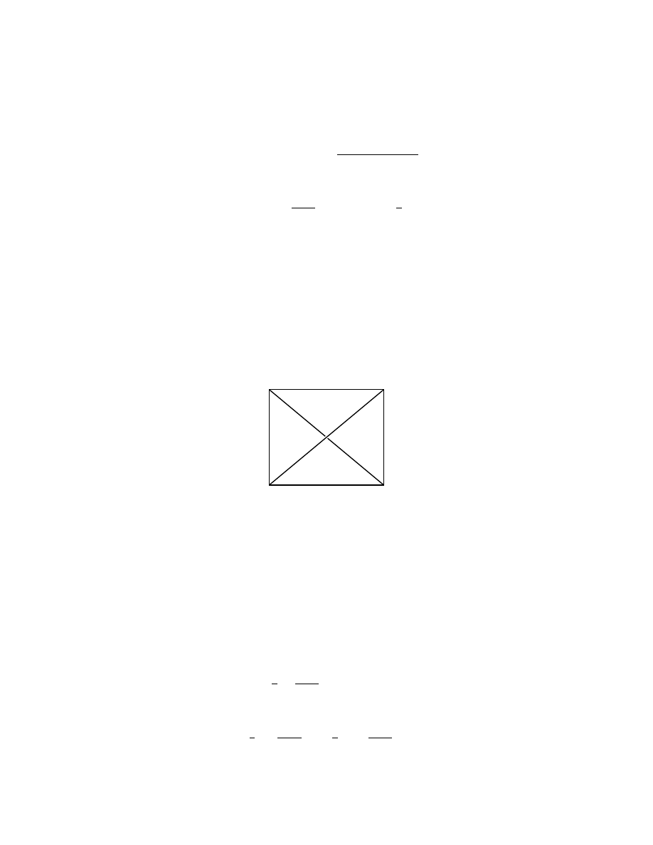
10. SCISSORS CONGRUENCE FOR HYPERBOLIC 3-MANIFOLDS
41
congruence by the cross ratio
z = [z
1
: z
2
: z
3
: z
4
] =
(z
3
− z
2
)(z
4
− z
1
)
(z
3
− z
1
)(z
4
− z
2
)
.
Permuting the vertices by an even (i.e., orientation preserving) permutation replaces
z by one of
z,
z
0
=
1
1 − z
,
or z
00
= 1 −
1
z
.
The parameter z lies in the upper half plane of C if the orientation induced by the
given ordering of the vertices agrees with the orientation of H
3
.
There is another way of describing the cross-ratio parameter z = [z
1
: z
2
: z
3
:
z
4
] of a simplex. The group of orientation preserving isometries of H
3
fixing the
points z
1
and z
2
is isomorphic to the multiplicative group C
∗
of nonzero complex
numbers. The element of this C
∗
that takes z
4
to z
3
is z. Thus the cross-ratio
parameter z is associated with the edge z
1
z
2
of the simplex. The parameter asso-
ciated in this way with the other two edges z
1
z
4
and z
1
z
3
out of z
1
are z
0
and z
00
respectively, while the edges z
3
z
4
, z
2
z
3
, and z
2
z
4
have the same parameters z, z
0
,
and z
00
as their opposite edges. See fig. 1. This description makes clear that the
dihedral angles at the edges of the simplex are arg(z), arg(z
0
), arg(z
00
) respectively,
with opposite edges having the same angle.
z4
z3
z2
z1
z
z
z´´
z´´
z´
z´
Figure 1
Now suppose we have five points z
0
, z
1
, z
2
, z
3
, z
4
∈ CP
1
= C ∪ {∞}. Any four-
tuple of these five points spans an ideal simplex, and the convex hull of these five
points decomposes in two ways into such simplices, once into two of them and once
into three of them. We thus get a scissors congruence relation equating the two
simplices with the three simplices. It is often called the “five term relation.” To
express it in terms of the cross-ratio parameters we need an orientation convention.
We allow simplices whose vertex ordering does not agree with the orientation
of H
3
(so the cross-ratio parameter is in the lower complex half-plane) but make
the convention that this represents the negative element in scissors congruence. An
odd permutation of the vertices of a simplex replaces the cross-ratio parameter z
by
1
z
,
z
z − 1
,
or 1 − z,
so if we denote by [z] the element in P(H
3
) represented by an ideal simplex with
parameter z, then our orientation rules say:
(4)
[z] = [1 −
1
z
] = [
1
1 − z
] = −[
1
z
] = −[
z − 1
z
] = −[1 − z].
42
3. ARITHMETIC INVARIANTS
Exercise 18. These orientation rules make the five-term scissors congruence
relation described above particularly easy to state:
4
X
i=0
(−1)
i
[z
0
: · · · : ˆ
z
i
: · · · : z
4
] = 0.
The cross ratio parameters occuring in this formula can be expressed in terms of
the first two as
[z
1
: z
2
: z
3
: z
4
] =: x
[z
0
: z
2
: z
3
: z
4
] =: y
[z
0
: z
1
: z
3
: z
4
] =
y
x
[z
0
: z
1
: z
2
: z
4
] =
1 − x
−1
1 − y
−1
[z
0
: z
1
: z
2
: z
3
] =
1 − x
1 − y
so the five-term relation can also be written:
(5)
[x] − [y] + [
y
x
] − [
1 − x
−1
1 − y
−1
] + [
1 − x
1 − y
] = 0.
We lose nothing if we also allow degenerate ideal simplices whose vertices lie
in one plane so the parameter z is real (we always require that the vertices are
distinct, so the parameter is in R − {0, 1}), since the five-term relation can be used
to express such a “flat” simplex in terms of non-flat ones, and one readily checks no
additional relations result. Thus we may take the parameter z of an ideal simplex
to lie in C − {0, 1} and every such z corresponds to an ideal simplex.
One can show that relations (4) follow from the five-term relation (5), so we
consider the quotient
P(C) := ZhC − {0, 1}i/(five-term relations (5))
of the free Z-module on C − {0, 1}. Proposition 10.3 can be restated that there is
a natural surjection P(C) → P(H
3
). In fact Dupont and Sah (loc. cit.) prove:
Theorem 10.4. The scissors congruence group P(H
3
) is the quotient of P(C)
by the relations [z] = −[z] which identify each ideal simplex with its mirror image.
Thus P(C) is a candidate for the orientation sensitive scissors congruence group
that we were seeking.
The analog of the Dehn invariant has a particularly elegant expression in these
terms. P(C) is known to be a Q-vector space and is therefore the sum of its ±1
eigenspaces under the map induced by complex conjugation. The above theorem
expresses P(H
3
) as the “imaginary part” P(C)
−
(negative eigenspace for complex
conjugation) of P(C).
Proposition/Definition 10.5. The Dehn invariant δ : P(H
3
) → R ⊗ R/πQ
is twice the “imaginary part” of the map
δ
C
: P(C) → C
∗
∧ C
∗
,
[z] 7→ (1 − z) ∧ z
so we shall call this map the “complex Dehn invariant.” We denote the kernel of
complex Dehn invariant
B(C) := Ker(δ
C
),
and call it the “Bloch group of C.”
Exercise 19. Compute the real and imaginary parts of the above δ
C
to confirm
the above proposition.

11. COMPUTING β(M )
43
A hyperbolic 3-manifold M has an “orientation sensitive scissors congruence
class” which lies in this Bloch group. The way one defines this is to subdivide M
3
into ideal tetrahedra. This cannot be done in the usual sense if M
3
is compact,
but it can be done in a weak sense which suffices for our purposes. We just require
a “degree one ideal triangulation” of M
3
, by which we mean that we should have
a collection of ideal simplices glued together by pairing faces plus a map of the
resulting “ideal complex” to M , locally isometric on each simplex, and of degree
one almost everywhere in M . It is not hard to show that such degree one ideal
triangulations exist (e.g., start from an ordinary “finite” triangulation by geodesic
simplices and then move vertices continuously off to infinity, taking care not to let
simplices degenerate).
Theorem 10.6 ([37]). Given a degree one ideal triangulation of a hyperbolic
manifold M
3
using simplices with cross-ratio parameters z
1
, . . . , z
n
say, the element
β(M ) := [z
1
] + · · · + [z
n
] ∈ P(C) is independent of the choice of triangulation and
lies in B(C).
Note that the definition of B(C) is purely algebraic, and so the same definition
could be made with C replaced by any subfield k.
Here are some facts about these groups which collate results of several people
(see [31] for detailed references).
Theorem 10.7. B(C) is a uniquely divisible group, so it has the natural struc-
ture of a Q-vector space. If k ⊂ C is a number field then B(k) → B(C) is injective
modulo torsion and has image isomorphic to Z
r
2
, where r
2
is the number of complex
embeddings of k. In particular, B(k)
Q
:= B(k) ⊗ Q is an r
2
-dimensional Q-vector-
subspace of B(C).
Theorem 10.8 ([37]). If M is a hyperbolic 3-manifold and k is the invariant
trace field of M , then β(M ) ∈ B(k)
Q
⊂ B(C).
11. Computing β(M )
Let D
2
be the so called “Bloch-Wigner dilogarithm function” given by:
D
2
(z) = Im ln
2
(z) + log |z| arg(1 − z),
z ∈ C − {0, 1},
where ln
2
(z) is the classical dilogarithm function. This function has geometric
meaning: D
2
(z) is the signed volume of the ideal simplex with cross-ratio parameter
z. It follows the map D
2
is compatible with the five-term relation and therefore
induces a map which we call vol from P(C) to R
If k is a number field with r
2
complex embeddings up to conjugation, let us list
these embeddings as σ
1
, . . . , σ
r
2
and denote
vol
i
:= vol ◦σ
i
: P(k) → R
Definition 11.1. The Borel regulator is the map
(vol
1
, . . . , vol
r
2
) : B(k) → R
r
2
.
Theorem 11.2 (Borel, Suslin). The Borel regulator maps B(k)/Torsion injec-
tively onto a full sublattice of R
r
2
.
This is the theorem which makes scissors congruence of hyperbolic 3-manifolds
computable. In fact, there is a computer program “snap” written by O. Goodman
using ingredients from Jeff Weeks’ program “snappea,” which does these compu-
tations (and much more). It is described in detail, along with several tables of

44
3. ARITHMETIC INVARIANTS
computations, in [9]. Both this paper and the actual program are available from
http://www.ms.unimelb.edu/˜snap.
We close these notes with one final exercise. We first remind that if k is an
imaginary quadratic number field, then 3-manifolds with invariant trace field k
do exist. In fact infinitely many non-commensurable ones do, since one can take
arithmetic manifolds with different quaternion algebras.
Exercise 20. Show that two hyperbolic 3-manifolds with imaginary quadratic
invariant trace fields are scissors congruence commensurable if and only if they have
the same invariant trace fields.
Contrast this exercise with the Dehn invariant sufficiency conjecture: that con-
jecture would imply that the volumes of two manifolds with different imaginary
quadratic invariant trace fields cannot be rational multiples of each other, but it is
not even proved that any volume of any hyperbolic 3-manifold is actually irrational!
12. Solution to Exercise 19
Consider the ideal tetrahedron ∆(z) with parameter z. We may position its
vertices at 0, 1, ∞, z. There is a Klein 4-group of symmetries of this tetrahedron
and it is easily verified that it takes the following horoballs to each other:
• At ∞ the horoball {(w, t) ∈ C × R
+
|t ≥ a};
• at 0 the horoball of euclidean diameter |z|/a;
• at 1 the horoball of euclidean diameter |1 − z|/a;
• at z the horoball of euclidean diameter |z(z − 1)|/a.
After truncation, the vertical edges thus have lengths 2 log a−log |z|, 2 log a−log |1−
z|, and 2 log a − log |z(z − 1)| respectively, and we have earlier said that their angles
are arg(z), arg(1/(1 − z)), arg((z − 1)/z) respectively. Thus, adding contributions,
we find that these three edges contribute log |1 − z| ⊗ arg(z) − log |z| ⊗ arg(1 − z)
to the Dehn invariant. By symmetry the other three edges contribute the same, so
the Dehn invariant is:
δ(∆(z)) = 2
¡
log |1 − z| ⊗ arg(z) − log |z| ⊗ arg(1 − z)
¢
∈ R ⊗ R/πQ.
On the other hand, to understand the “imaginary part” of (1 − z) ∧ z ∈ C
∗
∧ C
∗
we use the isomorphism
C
∗
→ R ⊕ R/2πZ,
z 7→ log |z| ⊕ arg z,
to represent
C
∗
∧ C
∗
= (R ⊕ R/2πZ) ∧ (R ⊕ R/2πZ)
= (R ∧ R) ⊕ (R/2πZ ∧ R/2πZ)
⊕
(R ⊗ R/2πZ)
= (R ∧ R) ⊕ (R/πQ ∧ R/πQ)
⊕
(R ⊗ R/πQ),
(the equality on the third line is because tensoring over Z with a divisible group is
effectively the same as tensoring over Q). Under this isomorphism we have
(1 − z) ∧ z =
¡
log |1 − z| ∧ log |z| ⊕ arg(1 − z) ∧ arg z
¢
⊕
¡
log |1 − z| ⊗ arg z − log |z| ⊗ arg(1 − z)
¢
,
confirming the Proposition 10.5.

APPENDIX A
Examples
In this appendix we will work through some explicit examples related to the
preceding notes. These were presented during tutorials at the Tur´an Workshop.
1. Trefoil complement
We will put two geometric structures on the trefoil complement. Since the
trefoil is a torus knot its complement is Seifert fibred with an orbifold quotient
F given by the disk with two orbifold points of orders 2 and 3. Thus χ(F ) =
1 − (1 − 1/2) − (1 − 1/3) = −1/6 so F admits a hyperbolic structure. We can realise
this explicitly with the orbifold given in example 4.2 of Chapter 1 of the notes,
F ∼
= P SL(2, Z)\H
2
. Now pull back the metric using the map S
3
− K → F . This
construction is not so explicit and in fact we can pull back the metric in different
ways to get H
2
× R structures or a PSL structure.
A better way to see things is as follows. We use the fact that the trefoil is a
fibred knot. This can be seen from the fundamental group
π
1
(S
3
− K) = {a
1
, a
2
, a
3
|a
1
a
2
= a
2
a
3
= a
3
a
1
}
∼
= {a, x, y|a
−1
xa = y, a
−1
ya = x
−1
y}
or as the link of the singularity Y
2
+ X
3
= 0. We can perturb this to Y
2
= −X
3
+ ²
which describes the Milnor fibre, or the Seifert surface S, of the trefoil as a branched
cover of the disk with branch points X
0
, ζX
0
, ζ
2
X
0
where ζ
3
= 1. This makes the
holonomy of the fibration S
3
− K → S
1
clear—it is given by rotation of the disk
by 2π/3.
Figure 1
Thus if we have a hyperbolic metric on the orbifold given by the disk with
degree 2 orbifold points at the branch points that is invariant under the holonomy
this gives an explicit H
2
× R structure on S
3
− K. Notice that if we quotient S by
the Z/3 action we get the orbifold F described above. The hyperbolic metric on
F lifts to a hyperbolic metric on S invariant under rotation by 2π/3 so we see the
H
2
× R structure explicitly.
We can also get the PSL structure as follows. If we put a left invariant metric
on P SL(2, R) then it pushes down to the quotient P SL(2, Z)\P SL(2, R). This
45
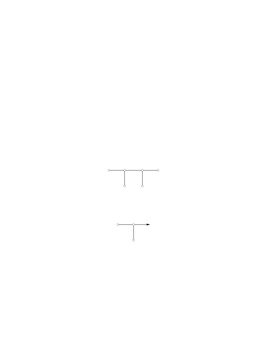
46
A. EXAMPLES
quotient is the complement of the trefoil. We can see this by studying the action
of SO(2) on the right and seeing that the quotient P SL(2, Z)\P SL(2, R)/SO(2) is
a disk with two orbifold points of degrees 2 and 3. By the classification of Seifert
fibred spaces this must be the trefoil complement. Notice that the Seifert surface
is totally geodesic in the H
2
× R case, but not so in the PSL case.
This example is one of the few cases when two types of geometries can be put
on the manifold. We cannot put a hyperbolic structure on the trefoil complement
due to the following general fact about Seifert fibred spaces. A fibre of the Seifert
fibring gives a normal Z in the fundamental group of the trefoil complement. Thus,
the square of any element of the fundamental group commutes with the element
represented by a fibre. This gives two parabolic elements and hence a cusp. But
there are more commuting parabolic elements and they also define the same cusp
which contradicts the fact that a lattice in the boundary C cannot have more than
two generators.
2. JSJ decomposition
We will give the JSJ decomposition of the link of the singularity
f = (x
2
+ y
3
)
2
+ xy
5
+ z
5
.
The plumbing graph of this link is given in the following appendix. It is equivalent
to the splice diagram in figure 2. See [15]. For this example it is sufficient to
5
2
5
3
2
13
Figure 2
understand the following fact about splice diagrams. The simplest type of splice
diagram is of the form in figure 3 which represents a Seifert fibred space with three
3
2
5
Figure 3
singular fibres of multiplicities 2, 3 and 5, respectively. The arrow indicates that
we wish to specify the singular fibre of multiplicity 5 as a link component in the
Seifert fibred space. (In this case the link is a knot.) The splice diagram in figure 2
is obtained by “splicing” together the Seifert fibred spaces represented in figures 3
and 4 along the two specified knots. We splice by removing a neighbourhood of
each knot and identifying the respective boundary tori where the longitude and
meridian of one torus is mapped to the meridian and longitude of the other torus.
This is exactly the canonical decompositon of the three-manifold into two
Seifert fibred spaces. They can each be given either the geometry H × R or PSL.
3. IDEAL TETRAHEDRA AND THE INVARIANT TRACE FIELD
47
5
2
13
Figure 4
3. Ideal tetrahedra and the invariant trace field
We will show that the invariant trace field of an ideally triangulated hyperbolic
manifold with cusps is generated by its tetrahedra parameters. See [32] for further
details.
Given M
3
non-compact and ideally triangulated notate its set of cusps by
C ⊂ ∂H
3
= C∪{∞}. Define k
∆
to be the field generated by the simplex parameters
of the ideal tetrahedra. Take one of the ideal tetrahedra of M
3
and put three of
the vertices of the tetrahedron at 0, 1 and ∞.
(i) First we will show that C ⊂ k
∆
∪ {∞} and C generates k
∆
∪ {∞}.
This is proved by induction using the fact that if three of z
1
, ...z
4
are in k
∆
∪{∞}
then the last one is in k
∆
∪{∞} if an only if the cross ratio is in k
∆
∪{∞}. Thus, we
begin with the tetrahedron with three vertices at 0, 1 and ∞ and use the preceding
fact to see that the fourth vertex lies in k
∆
∪ {∞}. Any ideal tetrahedron that
shares a face with this tetrahedron now has three of its vertices in k
∆
∪ {∞} so
the induction continues to this tetrahedron. Thus C ⊂ k
∆
∪ {∞} and C generates
k
∆
∪ {∞} since each simplex parameters is the cross ratio of four cusp points.
Thus it is sufficent to show that k
∆
= k(Γ).
(ii) k
∆
⊂ k(Γ).
Since Γ ⊂ k(Γ) · ¯
Γ = Q(Γ), the quaternion algebra associated to Γ, then the
existence of parabolic elements implies that Q(Γ) ⊂ M (2, C) has zero divisors—
if P is parabolic then (P − I)
2
= 0—so Q(Γ) ∼
= M (2, k(Γ)). Therefore we can
conjugate Γ to get a subgroup of P GL(2, k(Γ)). Notice that if g ∈ P GL(2, k(Γ))
then g
2
/det(g) ∈ P SL(2, k(Γ)) and thus we can conjugate Γ
(2)
to a subset of
P SL(2, k(Γ)). Now, a cusp is a solution of
µ
a b
c d
¶ µ
x
y
=
µ
x
y
where the matrix lies in P GL(2, k(Γ)) and in fact by using the square of an element
of Γ we may assume that the matrix lies in P SL(2, k(Γ)). Therefore x/y ∈ k(Γ).
(iii) If Γ is a group fixing a subset of k
∆
∪ {∞} then Γ ⊂ P GL(2, k
∆
).
We can see this simply by observing that the following equation:
γ =
µ
a b
c d
,
γ(0) = α
γ(1) = β
γ(∞) = γ
∈ k
∆
∪ {∞}.
has a solution in k
∆
:
b = αd, a + b = βc + βd, a = cγ.
Thus, Γ ⊂ P GL(2, k
∆
) and Γ
(2)
⊂ P SL(2, k
∆
) so it follows that k(Γ) ⊂ k
∆
.
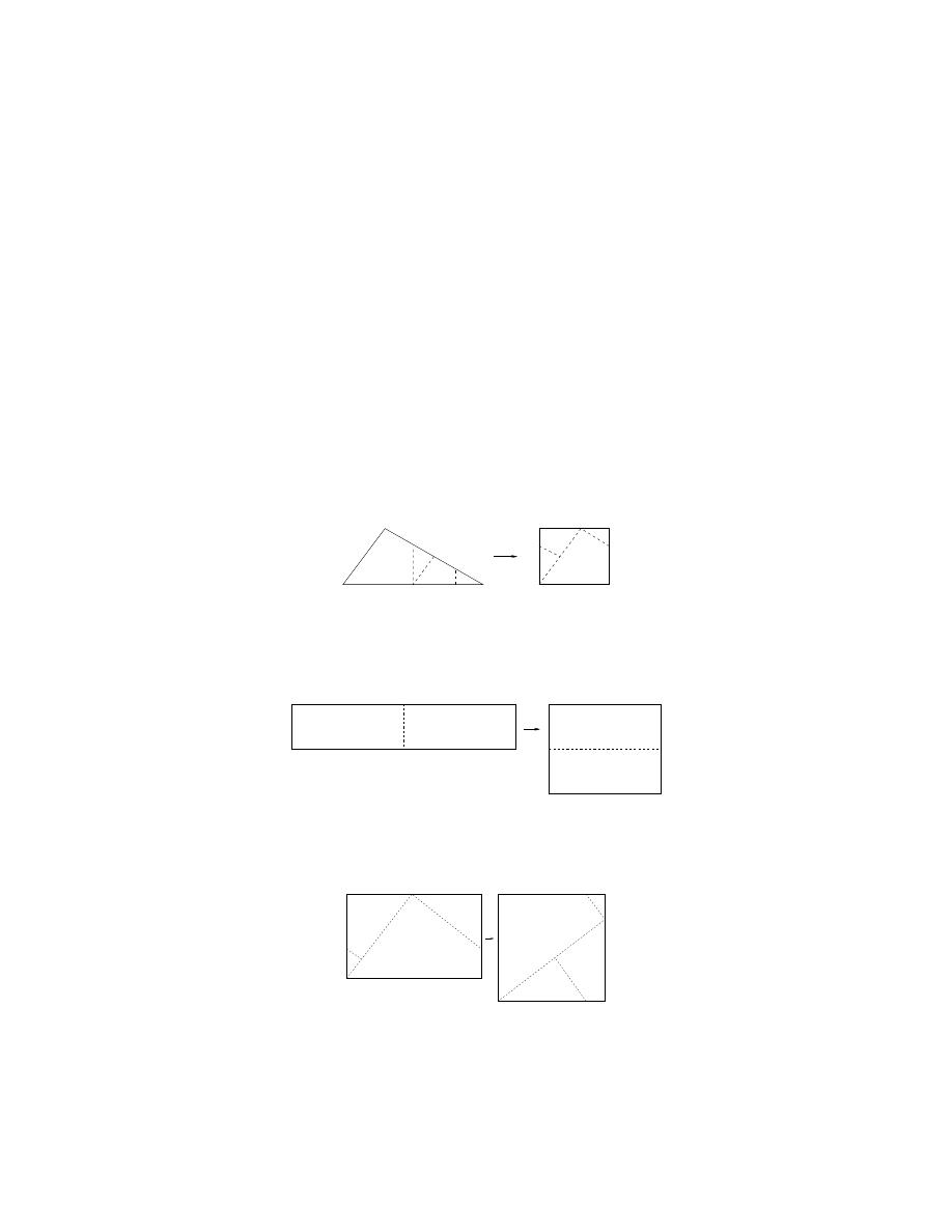
48
A. EXAMPLES
4. Scissors congruence
Here we will prove that two Euclidean polygons are scissors congruent if and
only if they have the same area.
Given two polygons of equal area we can reduce the problem of scissors con-
gruence to two equal area triangles as follows. Assume we can solve the equal area
triangle problem. Cut the two polygons into triangles and take a triangle from each
polygon. If they have equal area then we use the solution of the equal area triangle
problem to cut the two triangles into equal pieces. If they have unequal area then
cut the bigger one into two triangles one of which has the same area as the triangle
from the other polygon. (We can do this by the intermediate value theorem.) Now
cut the two equal area trangles into identical pieces. This has reduced the problem.
In the first case the total number of triangles is reduced by two and in the second
case the number is reduced by one.
Scissors congruence is an equivalence relation since we can cut a polygon further
to prove transitivity. Thus to solve the equal area triangle problem it is enough to
show that any triangle is scissors congruent to the square of equal area. From the
diagram we see how to go from a triangle to a rectangle.
Figure 5
To go from the rectangle to the square we cut the rectangle as shown until the
ratio of the two sides is not greater than two.
Figure 6
Then the following diagram gives the equivalence with the square.
Figure 7

APPENDIX B
Problems
The following set of problems were used during the Tur´an Workshop. They are
sometimes answered in the course notes and the worked examples.
1. Geometries
Quick
(i) Take a family of non-conjugate representations of π
1
Σ into SL(2, R). Does
Mostow-Prasad rigidity imply these representations are conjugate inside SL(2, C)?
(ii) Find all integer solutions {p
1
, ..., p
s
} of
2 − Σ
s
1
(1 − 1/p
i
) = 0 (= χ(F )).
(These give all flat compact genus 0 orbifolds, where the {p
i
} give the mulplicities
of the orbifold points.)
(iii) Put a hyperbolic structure on the surface of genus g.
Understanding
(i) Describe the complement of the trefoil in terms of the link of the singularity
y
2
= x
3
and hence describe the holonomy.
(ii) Put geometries on each of: the trefoil complement; figure-8 complement.
(iii) Why is the type of the geometry that can be put on a closed manifold
unique? (Hint: look for topological invariants.)
(iv) Describe the isometry groups of the 8 geometries in dimension 3.
(v) Describe the space of geodesics for each geometry.
Thoughtful
(i) Given any two Euclidean polygons of the same area, show that you can cut
one of them into a finite number of Euclidean polygons and reassemble the pieces
to get the other polygon.
(ii) We have seen that the trefoil complement admits a geometric structure
of type H
2
× R and also of type PSL. How can we see that it does not admit a
hyperbolic structure?
2. Decomposition
Quick
(i) What does an incompressible torus in Y
3
imply about the fundamental
group π
1
Y
3
? If the incompressible torus is boundary parallel what does this say in
terms of the fundamental group?
(ii) Give an example to show what is wrong with this definition:
an embedded annulus (A, ∂A) ,→ (Y, ∂Y ) is boundary parallel if there exists an
annulus ˜
A ⊂ ∂Y with ∂A = ∂ ˜
A and A ∪ ˜
A = ∂H for an embedded solid torus
H ,→ Y with H ∩ ∂Y = ˜
A.
(iii) Describe canonical circles in two dimensions.
49
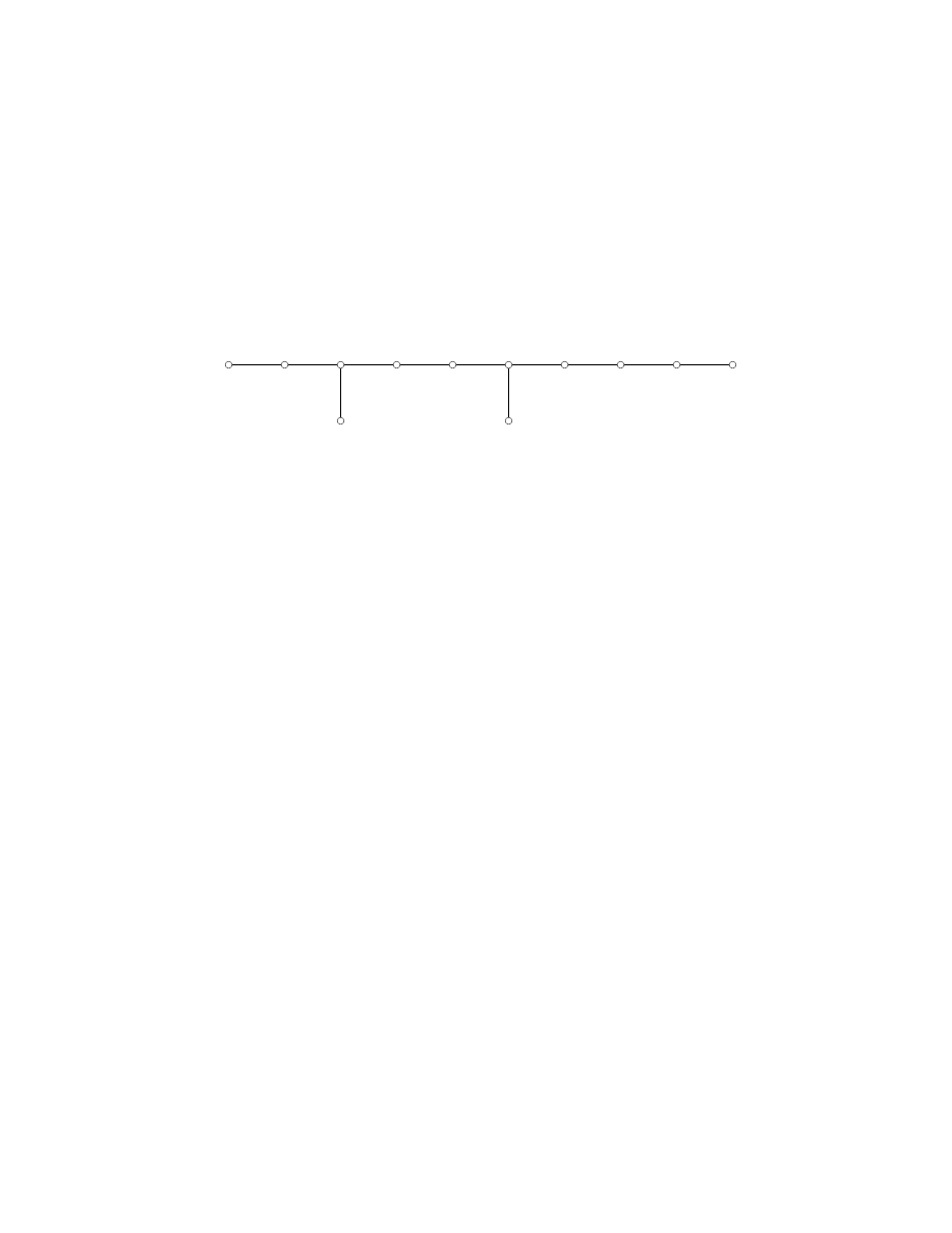
50
B. PROBLEMS
Understanding
(i) Find the maximal set of canonical tori, and hence the JSJ-decomposition, of
the following 3-manifolds: trefoil complement; figure-8 complement; trefoil cabled
on figure-8 complement; link of the singularity
f = (x
2
+ y
3
)
2
+ xy
5
+ z
5
.
(Hint: use the algorithm described in Nemethi’s course to verify that the resolution
of the singularity has plumbing graph
-2
-2
-2
-2
-2
-2
-2
-2
-2
-2
-3
-2
Figure 1
where each curve is a P
1
. Since the link is given by the boundary of a neighbourhood
of the divisor and hence a circle bundle over the smooth points of the divisor any
embedded circle in the divisor pulls back to a torus.)
Here are examples of decompositions where uniqueness fails:
(ii) Connect sum in two dimensions: prove that RP
2
#RP
2
#RP
2
∼
= T
2
#RP
2
.
(iii) Connect sum in three dimensions: Y ∼
= M
1
#M
2
#...#M
k
decomposes an
orientable 3-manifold Y into prime manifolds M
i
, unique up to order. What is not
unique here?
(iv) Connect sum of non-orientable 3-manifolds: give an example to show non-
uniqueness.
(v) Connect sum in four dimensions: give an example to show non-uniqueness.
(vi) What is the key point in the proof of uniqueness of JSJ-decompositions
that fails in the previous three cases. Show this explicitly with the example of the
blown up projective plane and torus (in (ii) above).
(vii) Show that every Seifert fibred space has a normal Z in its fundamental
group and thus a Seifert fibred space does not admit a hyperbolic structure.
(viii) Put a geometry on the torus with one orbifold point.
Thoughtful
(i) Canonical decomposition of maps of a surface: given a diffeomorphism f :
Σ → Σ, we say an embedded circle S
1
,→ Σ has finite order if some iterate of f
takes the circle to an istopic circle. Define a canonical circle to be a finite order
circle with the property that all other finite order circles can be isotoped off the
canonical circle. Use this to get a canonical decomposition of (Σ, f ) and show that
it is unique.
(ii) Given any two hyperbolic or spherical polygons of the same area, show that
you can cut one of them into a finite number of hyperbolic, respectively spherical,
polygons and reassemble the pieces to get the other polygon.
(iii) Prove that if both cos θ and θ/π are rational then θ is a multiple of π/2 or
π/3.

COMMENSURABILITY
51
Scissors congruence
Quick
(i) Show that scissors congruence is an equivalence relation.
(ii) Show R ⊗
Z
R/Z ∼
= R ⊗
Q
R/Q.
(iii) Calculate the Dehn invariant of the Euclidean polyhedron δ(Σ × I) for any
2-dimensional polygon Σ.
(iv) What is the Dehn invariant in dimension 2 (Euclidean, hyperbolic and
spherical) and why doesn’t it obstruct scissors congruence?
Understanding
(i) Prove that Euclidean polygons of the same area are scissors congruent:
(a) show that it is enough to prove this for two triangles;
(b) show that a triangle is scissors congruent to a rectangle;
(c) show that any rectangle is scissors congruent to a square;
(d) conclude the equivalence of any two polygons of equal area.
(ii) Prove that the Dehn invariant doesn’t vanish on a regular tetrahedron and
create your own example with δ 6= 0.
(iii) Prove: im(vol| ker δ) = R and im(δ| ker vol) = im(δ).
(iv) Recall that scissors congruence for finite area hyperbolic polygons with
ideal vertices is allowed. Show that stable scissors congruence is not the same as
scissors congruence. Show that two polygons are scissors congruent if and only if
they have the same area and they are either both compact or both non-compact
and stably scissors congruent if and only if they have the same area.
Thoughtful
(i) Where does the argument that Euclidean polygons of the same area are
scissors congruent (in Understanding(i) above) fail for hyperbolic and spherical
geometry? Can it be fixed?
(ii) Where does the argument that Euclidean polygons of the same area are
scissors congruent (in Understanding(i) above) fail in dimension 3? Does it succeed
on a limited class of polyhedra?
(iii) Show that for polygons P and Q, 2P ∼ 2Q implies P ∼ Q. Since this
is a general fact in any dimension and geometry, one can argue without using the
equality of area.
(iv) Define a Dehn invariant in dimension 4. Is it unique?
Commensurability
Quick
(i) Show that all ideal triangles in H
2
are isometric.
(ii) Show that not all ideal tetrahedra in H
3
are isometric.
(iii) Construct a rotation of R
2
that acts on Z[i] giving a commensurable lattice.
Show that a dense set of rotations has this property.
Understanding
(i) Show that the group of symmetries of the tessellation of H
3
by ideal tetra-
hedra is arithmetic.
(ii) Show that Comm
+
(P SL(2, Z[i])) = P GL(2, Q[i]).
(iii) Prove that there are exactly two quaternion algebras over R.
(iv) Show that the figure 8 knot and the Whitehead link are arithmetic.
Thoughtful
(i) Does arithmeticity exist in dimension 2?

52
B. PROBLEMS
Bloch group.
Quick
(i) Show explicitly that the figure 8 knot lies in the kernel of the complex Dehn
invariant. (Hint: the parameter for the figure 8 knot is given by 2[ζ] where ζ
6
= 1.)
(ii) Does hyperbolic Dehn surgery on the figure 8 knot change its scissors con-
gruence class in the Bloch group, β
0
(Y ) ∈ B(C)?
(iii) Are the hyperbolic Dehn surgeries on the figure 8 knot arithmetic?
Understanding
(i) Show that the invariant trace field of an ideally triangulated hyperbolic
manifold with cusps is generated by its tetrahedra parameters.
(ii) Show that two hyperbolic 3-manifolds with imaginary quadratic trace field
are scissors congruent commensurable if and only if they have the same invariant
trace fields.
(iii) Prove that the five-term scissors congruence relation implies that [z] =
[1 − 1/z].

Bibliography
[1] Adams, C., Limit volumes of hyperbolic three-orbifolds. J. Differential Geom. 34 (1991), no.
1, 115–141.
[2] Adams, C., Non-compact hyperbolic 3-orbifolds of small volume. Topology 90, Proceedings
of the Research Semester in Low Dimensional Topology at Ohio State, (Walter de Gruyter
Verlag, Berlin - New York 1992), 1–16.
[3] I. R. Aitcheson, and J. H. Rubinstein, Combinatorial cubings, cusps and the dodecahedral
knots. Topology 90, Proceedings of the Research Semester in Low Dimensional Topology at
Ohio State, (Walter de Gruyter Verlag ,Berlin - New York 1992), 17–26.
[4] M. B¨
okstedt, M. Brun, J.L. Dupont, Homology of O(n) and O
1
(1, n) made discrete: an
application of edgewise subdivision, J. Pure Appl. Algebra (to appear).
[5] Borel, A., Commensurability classes and volumes of hyperbolic 3-manifolds. Ann. Scuola
Norm. Sup. Pisa 8 (1981), 1–33.
[6] Chinburg, T. and Friedman, E., The smallest arithmetic hyperbolic 3-orbifold, Invent. Math.
86 (1986), 507–527.
[7] Chinburg, T., Jones, K.N. Friedman, E., Reid, A.W., The arithmetic hyperbolic 3-manifold
of smallest volume, Preprint 1998.
[8] In preparation.
[9] Coulson, D., Goodman, O.A., Hodgson, C.D. and Neumann, W.D., Computing arithmetic
invariants of 3-manifolds
[10] M.Dehn: ¨
Uber die Topologie des dreidimensionalen Raumes. Math. Ann. 69 (1910), 137–168.
[11] J.L. Dupont, The dilogarithm as a characteristic class for flat bundles, J. Pure and App.
Algebra 44 (1987), 137–164.
[12] J.L. Dupont, H. Sah, Scissors congruences II, J. Pure and App. Algebra 25 (1982), 159–195.
[13] J.L. Dupont, H. Sah, Homology of Euclidean groups of motions made discrete and Euclidean
scissors congruences, Acta Math. 164 (1990), 1–27.
[14] J.L. Dupont, H. Sah, Three questions about simplices in spherical and hyperbolic 3-space,
preprint 1997.
[15] D. Eisenbud and W.D. Neumann: Three-Dimensional Link Theory and Invariants of Plane
Curve Singularities, Annals of Math. Studies 110 (Princeton Univ. Press 1985).
[16] M. Freedman. J. Hass, P. Scott: Least area incompressible surfaces in 3-manifolds. Invent.
Math. 71 (1983), no. 3, 609–642.
[17] D. Gabei, G.R. Meyerhoff, N. Thurston, Homotopy hyperbolic manifolds are hyperbolic,
preprint 1996.
[18] A.B. Goncharov: Volumes of hyperbolic manifolds and mixed Tate motives, preprint MPI/96-
10 (Max-Planck-Institut f¨
ur Math., Bonn, 1996).
[19] D. Hilbert, Mathematical Problems, English translation in Mathematical developements aris-
ing from Hilbert’s problems, Proc. Symp. Pure Math. 28 part 1 (Amer. Math. Soc., 1976).
[20] W.H. Jaco and P.B. Shalen: Seifert fibered spaces in 3-manifolds, Memoirs of American
Math.Soc., Vol. 21, Number 220 (1979).
[21] W.H. Jaco: Lectures on Three-Manifold Topology, Amer. Math. Soc. Regional Conference
Series in Mathematics, 43 (1980).
[22] B. Jessen, The algebra of polyhedra and the Dehn-Sydler theorem, Math. Scand. 22 (1968),
241–256.
[23] B. Jessen, Zur Algebra der Polytope, G¨
ottinger Nachr. Math. Phys. (1972), 47–53.
[24] K. Johannson: Homotopy equivalences of 3-manifolds with boundary, Lecture Notes in Math-
ematics 761 (Springer-Verlag, 1979).
[25] J. Hempel: 3-Manifolds, Ann. of Math. Studies 86 (Princton Univ. Press, 1976).
53

54
BIBLIOGRAPHY
[26] Meyerhoff, R., A lower bound for the volume of hyperbolic 3-orbifolds. Duke Math. J. 57
(1988), 185–203.
[27] Milnor, J., A unique factorization theorem for 3-manifolds, Amer. J. Math. 84 (1962), 1–7.
[28] J. Milnor, Hyperbolic geometry: the first 150 years, Bulletin Amer. Math. Soc. 6 (1982),
9–24.
[29] Morgan, J. W. and Bass, H, eds, The Smith Conjecture, (Academic Press 1984).
[30] Neumann, W.D., Geometry of quasihomogeneous surface singularities, Singularities, Arcata
1981, Proc. Symp. Pure Math. 40 (Amer. Math. Soc. 1983), 244–258.
[31] Neumann, W.D., Hilbert’s 3rd Problem and invariants of 3-manifolds (solicited for
the David Epstein 60th Birthday volume of Geometry and Topology, preprint at
http://www.maths.mu.oz.au/ neumann).
[32] Neumann, W.D. and Reid, A.W., Notes on Adams’ small volume orbifolds. Topology 90,
Proceedings of the Research Semester in Low Dimensional Topology at Ohio State, (Walter
de Gruyter Verlag, Berlin - New York 1992), 273–310.
[33] Neumann, W.D. and Reid, A.W., Arithmetic of hyperbolic 3-manifolds, Topology 90, Pro-
ceedings of the Research Semester in Low Dimensional Topology at Ohio State, (Walter de
Gruyter Verlag, Berlin - New York 1992), 273–310.
[34] W.D. Neumann and G.A. Swarup: Canonical decompositions of 3-manifolds, Geometry and
Topology 1 (1997), 21–40.
[35] Neumann, W.D. and Jun Yang: Rationality Problems for K-theory and Chern-Simons In-
variants of Hyperbolic 3-Manifolds, Enseignement Math´ematique 41 (1995), 281–296.
[36] Neumann, W.D. and Jun Yang: Invariants from triangulations of hyperbolic 3-manifolds,
Electronic Research Announcements of the Amer. Math. Soc. 1 (2) (1995), 72–79.
[37] Neumann, W.D. and Jun Yang: Bloch invariants of hyperbolic 3-manifolds, Duke Math. J. 96
(1998) (to appear, electronic preprint available at http://www.maths.mu.oz.au/˜neumann).
[38] Neumann, W.D. and Zagier, D., Volumes of hyperbolic 3-manifolds. Topology 24 (1985),
307–332.
[39] C.S. Sah, Hilbert’s Third Problem: Scissors Congruence, Res. Notes in Math. 33 (Pitman,
1979).
[40] C. S. Sah, Scissors congruences, I, Gauss-Bonnet map, Math. Scand. 49 (1982) 181–210.
[41] G.P. Scott, The geometries of 3-manifolds, Bull. London Math. Soc. 15 (1983), 401–478.
[42] G.P. Scott: Strong annulus and torus theorems and the enclosing property of characteristic
submanifolds of 3-manifolds, Quarterly J. Math. Oxford (2), 35 (1984), 485–506,
[43] J. Stallings: On the loop theorem, Ann. of Math. 72 (1960), 12–19.
[44] A. A. Suslin, Algebraic K-theory of fields, Proc. Int. Cong. Math. Berkeley 86, vol. 1 (1987),
222–244.
[45] G. A. Swarup, On incompressible surfaces in the complements of knots. J. Indian Math. Soc.
(N.S.) 37 (1973), 9–24. Addendum: J. Indian Math. Soc. (N.S.) 38 (1974) 411–413.
[46] Thurston, W.P., The geometry and topology of 3-manifolds. Mimeographed lecture notes,
Princeton Univ., 1977.
[47] F. Waldhausen: On irreducible 3-manifolds which are sufficiently large. Ann. of Math. (2) 87
(1968), 56–88.
[48] F. Waldhausen: Gruppen mit Zentrum und 3-dimensionale Mannigfaltigkeiten, Topology 6
(1967), 505–517.
[49] F. Waldhausen: On the determination of some 3-manifolds by their fundamental groups alone,
Proc. of Inter. Sympo. Topology, Hercy-Novi, Yugoslavia, 1968, Beograd (1969), 331–332.
[50] F. Waldhausen: On some recent results in 3-dimensional topology, Proc. Symp. in Pure Math.
Amer. Math. Soc. 32 (1977), 21–38.
[51] D. Zagier, Polylogarithms, Dedekind zeta functions and the algebraic K-theory of fields.
Arithmetic algebraic geometry (Texel, 1989), Progr. Math., 89, (Birkh¨
auser Boston, Boston,
MA, 1991), 391–430.
[52] Zimmer, R., Ergodic Theory and Semi-simple Lie groups. Birkhauser, Boston, 1984.
Wyszukiwarka
Podobne podstrony:
(ebook martial arts) Wing Chun Kung Fu Breathing NOTES ON MEDITATION AND HEALTH
Gardner Differential geometry and relativity (lecture notes, web draft, 2004) (198s) PGr
EN Mahr General notes on form and location tolerances
Before the Day Breaks Conversations and Correspondence with Einstein by Immanuel Velikovsky
Novikov S P Solitons and geometry (Lezioni Fermiane, Cambridge Univ Press, 1994, web draft, 1993)(50
Ziming Li Lecture notes on computer algebra (web draft, 2004)(31s) CsCa
Rajeev S G Geometrical methods in physics (lecture notes, web draft, 2004)(97s)
An exegetical study on Divorce and Remarriage (Matt 19 9) by John Murray
Dynkin E B Superdiffusions and Positive Solutions of Nonlinear PDEs (web draft,2005)(108s) MCde
Brizard A J Introduction to Lagrangian and Hamiltonian mechanics (web draft, 2004)(173s) PCtm
A NEW CATALOGUE OF THE CERAMBYCIDAE (COLEOPTERA) OF ISRAEL WITH NOTES ON THEIR DISTRIBUTION AND HOST
Notes on the 3 inch gun materiel and field artillery equipment 1917
Lumiste Betweenness plane geometry and its relationship with convex linear and projective plane geo
Lumiste Tarski's system of Geometry and Betweenness Geometry with the Group of Movements
Notes on Basic 3 Manifold Topol Nieznany
Meziani A On first and second order planar elliptic equations with degeneracies (MEMO1019, AMS, 2012
Correspondence of Roosevelt and Truman with Stalin on Lend Lease and Other Aid to the Soviet Union
więcej podobnych podstron