
Chapter 15
AC Motor Speed Control
T.A. Lipo
Karel Jezernik
University of Wisconsin
University of Maribor
Madison WI, U.S.A
Maribor Slovenia
15.1 Introduction
An important factor in industrial progress during the past five decades has been
the increasing sophistication of factory automation which has improved pro-
ductivity manyfold. Manufacturing lines typically involve a variety of variable
speed motor drives which serve to power conveyor belts, robot arms, overhead
cranes, steel process lines, paper mills, and plastic and fiber processing lines to
name only a few. Prior to the 1950s all such applications required the use of a
DC motor drive since AC motors were not capable of smoothly varying speed
since they inherently operated synchronously or nearly synchronously with the
frequency of electrical input. To a large extent, these applications are now ser-
viced by what can be called general-purpose AC drives. In general, such AC
drives often feature a cost advantage over their DC counterparts and, in addi-
tion, offer lower maintenance, smaller motor size, and improved reliability.
However, the control flexibility available with these drives is limited and their
application is, in the main, restricted to fan, pump, and compressor types of
applications where the speed need be regulated only roughly and where tran-
sient response and low-speed performance are not critical.
More demanding drives used in machine tools, spindles, high-speed eleva-
tors, dynamometers, mine winders, rolling mills, glass float lines, and the like
have much more sophisticated requirements and must afford the flexibility to
allow for regulation of a number of variables, such as speed, position, acceler-
ation, and torque. Such high-performance applications typically require a high-
speed holding accuracy better than 0.25%, a wide speed range of at least 20:1,
and fast transient response, typically better than 50 rad/s, for the speed loop.
Until recently, such drives were almost exclusively the domain of DC motors
combined with various configurations of AC-to-DC converters depending
upon the application. With suitable control, however, induction motor drives

2
AC Motor Speed Control
Draft Date: February 5, 2002
have been shown to be more than a match for DC drives in high-performance
applications. While control of the induction machine is considerably more
complicated than its DC motor counterpart, with continual advancement of
microelectronics, these control complexities have essentially been overcome.
Although induction motors drives have already overtaken DC drives during the
next decade it is still too early to determine if DC drives will eventually be rel-
egated to the history book. However, the future decade will surely witness a
continued increase in the use of AC motor drives for all variable speed applica-
tions.
AC motor drives can be broadly categorized into two types, thyristor based
and transistor based drives. Thyristors posses the capability of self turn-on by
means of an associated gate signal but must rely upon circuit conditions to turn
off whereas transistor devices are capable of both turn-on and turn-off.
Because of their turn-off limitations, thyristor based drives must utilize an
alternating EMF to provide switching of the devices (commutation) which
requires reactive volt-amperes from the EMF source to accomplish.
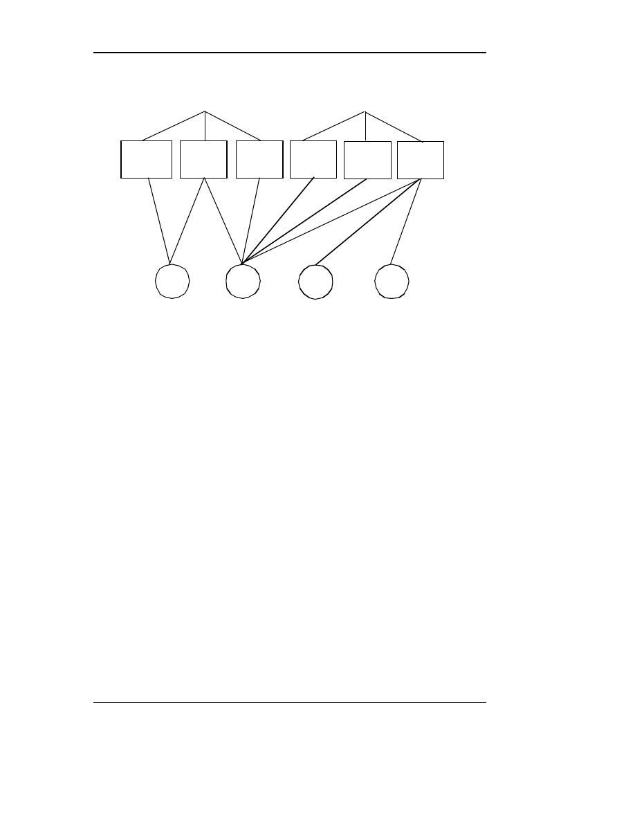
A brief list of the available drive types is given in Figure 15.1. The drives
are categorized according to switching nature (natural or force commutated),
converter type and motor type. Naturally commutated devices require external
voltage across the power terminals (anode-cathode) to accomplish turn-off of
the switch whereas a force commutated device uses a low power gate or base
voltage signal which initiates a turn-off mechanism in the switch itself. In this
figure the category of transistor based drives is intended to also include other
hard switched turn-off devices such as GTOs, MCTs and IGCTs which are, in
reality, avalanche turn-on (four-layer) devices.
The numerous drive types associated with each category is clearly exten-
sive and cannot be treated in complete detail here. However, the speed control
of the four major drive types having differing control principles will be consid-
ered namely 1) voltage controlled induction motor drives 2) load commutated
synchronous motor drives, 3) volts per hertz and vector controlled induction
motor drives and 4) vector controlled permanent magnet motor drives. The
control principles of the remaining drives of Figure 15.1 are generally straight-
forward variations of one of these four drive types.
Thyristor Based Voltage Controlled Drives
3
Draft Date: February 5, 2002
15.2 Thyristor Based Voltage Controlled Drives
15.2.1
Introduction
During the middle of the last century, limitations in solid state switch technol-
ogy hindered the performance of variable frequency drives. In what was essen-
tially a stop-gap measure, variable speed was frequently obtained by simply
varying the voltage to an induction motor while keeping the frequency con-
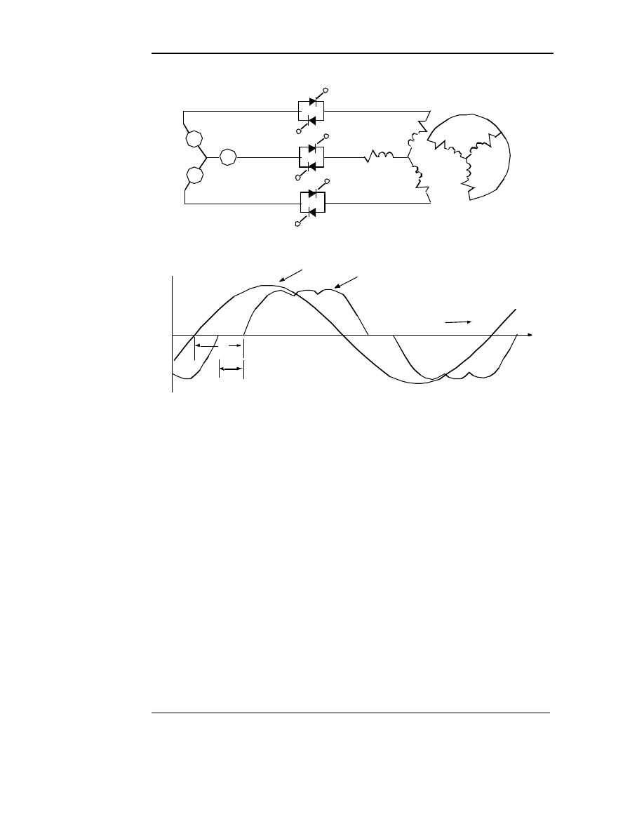
stant. The switching elements used were generally back-to-back connected
thyristors as shown in Figure 15.2. These devices were exceptionally rugged
compared to the fragile transistor devices of this era.
15.2.2
Basic Principles of Voltage Control
The basic principles of voltage control can be obtained readily from the con-
ventional induction motor equivalent circuit shown in Figure 15.3 and the
Figure 15.1 Major drive type categories
Thyristor Based Drives
Transistor Based Drives
Six Pulse
Bridge
Cyclo-
converter
Thyristor
Voltage
Controller
Matrix
Converter
Current
Link
PWM
Voltage
Link
PWM
Synchronous
Motor
Induction
Motor
Permanent
Magnet
Motor
Variable
Reluctance
Motor
Current Link
4
AC Motor Speed Control
Draft Date: February 5, 2002
associated constant voltage speed-torque curves illustrated in Figure 15.4. The
torque produced by the machine is equal to the power transferred across the
airgap divided by synchronous speed,
(15.1)
where P = number of poles, S is the per unit slip,
ω
e
is line frequency and I
2
, r
2
are the rotor rms current and rotor resistance respectively.
The peak torque points on the curves in Figure 15.4 occur when maximum
power is transferred across the airgap and are easily shown to take place at a
slip,
(15.2)
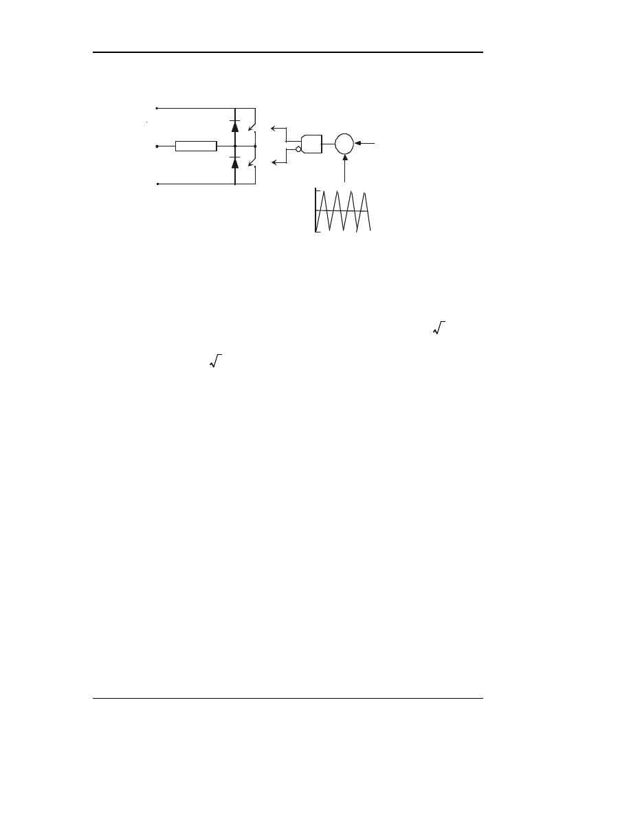
Figure 15.2
Induction motor voltage controller employing inverse-parallel
thyristors and typical current waveform
T1
T4
T3
T6
T2
T 5
i
b s
i
as
i
cs
v
as
v
cs
v
bs
i
as
AC Supply
s
a
b
c
+
+
+
e
a
′
g
ω
e
t
α
γ
Thyristor
Group
Induction Motor
e
a
′
g
e
b
′
g
e
c
′
g
g
a
′
c
′
b
′
T
e
3
2
--- P
I
2
2
r
2
S
ω
e
---------
=
S
MaxT
r
2
x
1
x
2
+
----------------
≈
Thyristor Based Voltage Controlled Drives
5
Draft Date: February 5, 2002
where x
1
and x
2
are the stator and rotor leakage reactances. From these results
and the equivalent circuit, the following principles of voltage control are evi-
dent:
(1) For any fixed slip or speed, the current varies directly with voltage and
the torque and power with voltage squared.
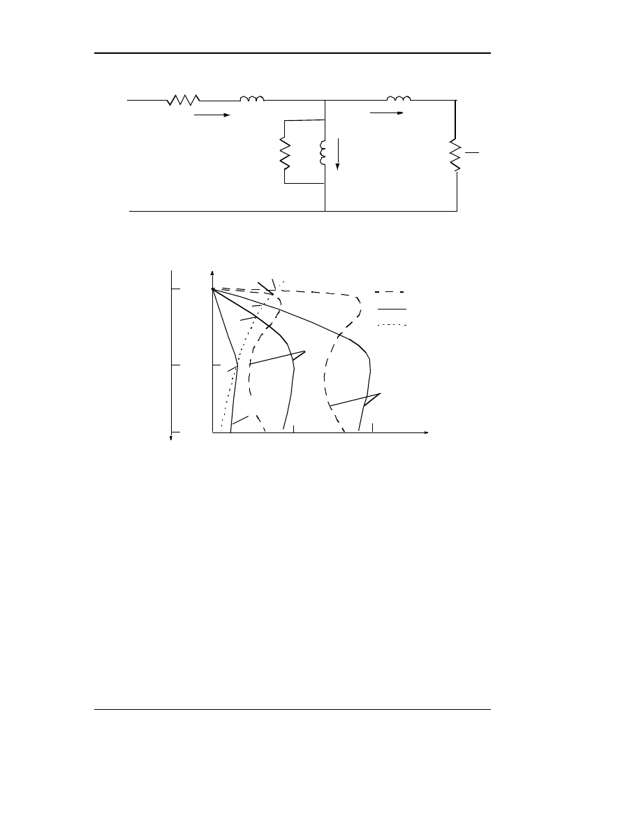
(2) As a result of (1) the torque-speed curve for a reduced voltage maintains
its shape exactly but has reduced torque at all speeds, see Figure 15.4.
(3) For a given load characteristic, a reduction in voltage will produce an
increase in slip (from A to A' for the conventional machine in Figure 15.4,
for example).
Figure 15.3
Per phase equivalent circuit of a squirrel cage induction
machine
r
2
S
jx
2
jx
1
r
1
I
2
I
1
V
1
+
–
r
m
I
m
jx
m
~
~
~
~
Figure 15.4
Torque versus speed curves for standard and high slip
induction machines
Standard Motor
High Slip Motor
Load Characteristic
V1= 1.0
V1= 0.7
A
0
0
0.5
1.0
0
0.5
1.0
B
S
li
p
(
p
er
u
n
it
)
S
p
e
ed
(
p
er
u
n
it
)
Torque (per unit)
1.0
2.0
A
′
B
′
B
′′
V1= 0.4

6
AC Motor Speed Control
Draft Date: February 5, 2002
(4) A high-slip machine has relatively higher rotor resistance and results in a
larger speed change for a given voltage reduction and load characteristic
(compare A to A' with B to B' in Figure 15.4).
(5) At small values of torque, the slip is small and the major power loss is
the core loss in r
m
. Reducing the voltage will reduce the core loss at the
expense of higher slip and increased rotor and stator loss. Thus there is
an optimal slip which maximizes the efficiency and varying the voltage can
maintain high efficiency even at low torque loads.
15.2.3
Converter Model of Voltage Controller
It has been shown that a very accurate fundamental component model for a
voltage converter comprised of inverse parallel thyristors (or Triacs) is a series
reactance given by [1]:
(15.3)
where and are the induction motor sta-
tor leakage, rotor leakage and magnetizing reactances respectively and is the
thyristor hold-off angle identified in Figure 15.2 and
(15.4)
This reactance can be added in series with the motor equivalent circuit to
model a voltage-controlled system. For typical machines the accuracy is well
within acceptable limits although the approximation is better in larger
machines and for smaller values of . In most cases of interest, the error is
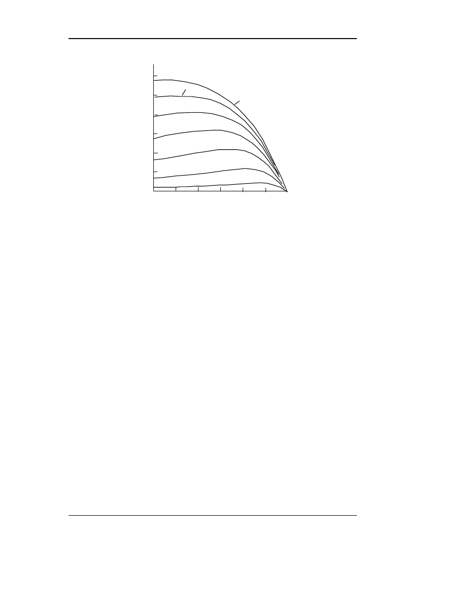
quite small. However, the harmonic power losses and torque ripple produced
by the current harmonics implied in Figure 15.2 are entirely neglected. A plot
of typical torque versus speed characteristics as a function of is shown in
Figure 15.5 for a 0.4 hp squirrel cage induction machine [2].
15.2.4
Speed Control of Voltage Controlled Drive
Variable-voltage speed controllers must contend with the problem of greatly
increased slip losses at speeds far from synchronous and the resulting low effi-
ciency. In addition, only speeds below synchronous speed are attainable and
speed stability may be a problem unless some form of feedback is employed.
I
2
r
x
eq
x
s
′
f
γ
( )
=
x
s
′
x
1
x
2
x
m
x
2
x
m
+
(
)
⁄
+
=
x
1
x
2
x
m
, ,
γ
f
γ
( )
3
π
---
γ
γ
sin
+
(
)
1
3
π
---
γ
γ
sin
+
(
)
–
-------------------------------------
=
γ
γ
Thyristor Based Voltage Controlled Drives
7
Draft Date: February 5, 2002
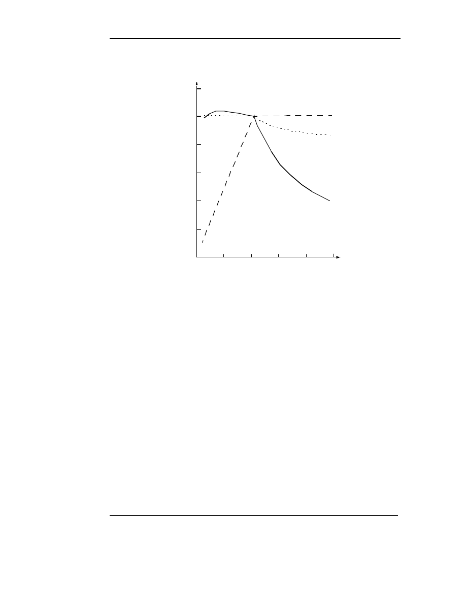
An appreciation of the efficiency and motor heating problem is available
from Equation (15.1) rewritten to focus on the rotor loss,
(15.5)
Thus the rotor copper loss is proportional not only to the torque but also to the
slip (deviation from synchronous speed). The inherent problem of slip varia-
tion for speed control is clearly indicated.
As a result of the large rotor losses to be expected at high slip, voltage con-
trol is only applicable to loads in which the torque drops off rapidly as the
speed is reduced. The most important practical case is fan speed control in
which the torque required varies as the speed squared. For this case, equating
the motor torque to the load torque results in:
(15.6)
Solving for
as a function of S and differentiating yields the result that the
maximum value of
(and hence of rotor loss) occurs at:
(15.7)
Figure 15.5 Torque speed curves for changes in hold off angle
γ
300
600
900
1200
1500
1800
60
o
50
o
40
o
30
o
20
o
γ
= 0
γ
= 10
o
1.0
2.0
3.0
4.0
5.0
6.0
A
v
er
a
g
e
T
o
rq
u
e
(N
.m
)
Rotor Speed (rev/min)
I
2
r
3I
2
2
r
2
SP
gap
S
2
P
---
ω
e
T
e
=
=
3
2
--- P
I
2
2
r
2
S
ω
e
---------
K
L
ω
e
1
S
–
(
)
2
=
I
2
2
I
2
2
S
1 3
⁄
=
8
AC Motor Speed Control
Draft Date: February 5, 2002
or at a speed of two-thirds of synchronous speed. If this worst case value is
substituted back to find the maximum required value of
and the result used
to relate the maximum rotor loss to the rotor loss at rated slip, the result is
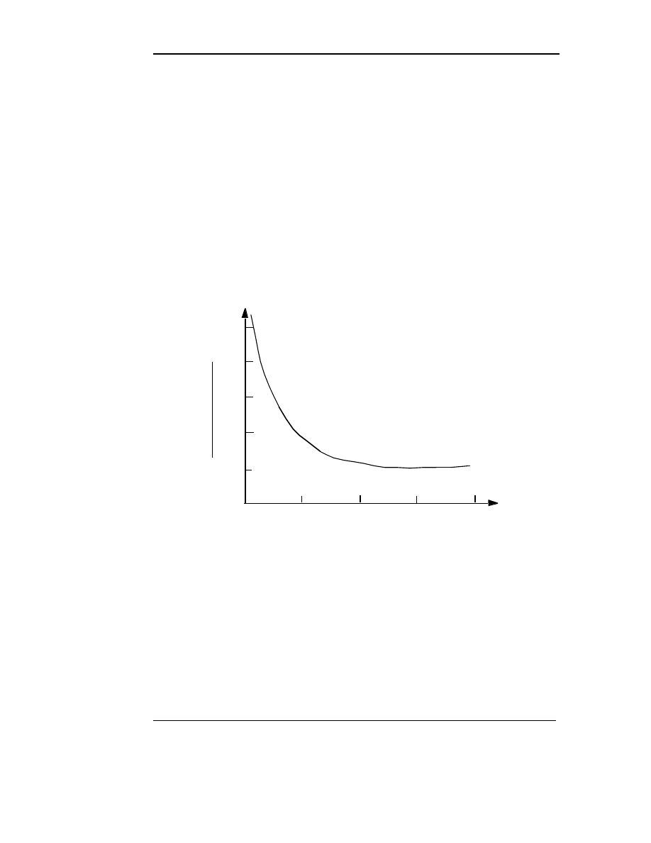
(15.8)
where S
rated
equals rated slip. Figure 15.6 illustrates this result and from this
curve it is clear that, to avoid excessive rotor heating at reduced speed with a
fan load, it is essential that the rated slip be in the range 0.25 – 0.35 to avoid
overheating. While the use of such high slip machines will avoid rotor over-
heating, it does not improve the efficiency. The low efficiency associated with
high slip operation is inherent in all induction machines and the high slip losses
implies that these machine will generally be large and bulky.
As noted previously, speed stability is an inherent problem in voltage-con-
trolled induction motor drives at low speeds. This is a result of the near coinci-
dence of the motor torque characteristic and the load characteristic at low
speed. The problem occurs primarily when the intersection of the motor torque
characteristic and the load characteristic occurs near or below the speed of
maximum motor torque (see point B in Figure 15.5).
Reduced voltage operation of an induction machine will result in lower
speed but this requires increased slip and the rotor I
2
r losses are accordingly
I
2
2
Maximum rotor I
2
r loss
Rated rotor I
2
r loss
----------------------------------------------------------
4 27
⁄
(
)
S
rated
1
S
rated
–
(
)
-----------------------------------------
=
Figure 15.6
Worst case rotor heating for induction motor with a fan load
5
4
3
2
1
0
0
0.1
0.2
0.3
0.4
Rated Slip S
R
M
a
x
im
u
m
R
o
to
r
I
2
r
R
a
te
d
R
o
to
r
I
2
R

Thyristor Based Load-Commutated Inverter Synchronous Motor Drives
9
Draft Date: February 5, 2002
increased. This type of high slip drive is therefore limited in application to sit-
uations where the high losses and low efficiency are acceptable and, generally,
where the speed range is not large. Such drives are today generally limited to
relatively low power ratings because of cooling problems.
The voltage controller of Figure 15.2, however, remains popular for motor
starting applications. Motor starters are intended to provide a reduction in start-
ing current. Inverse parallel thyristor starters reduce the current by the voltage
ratio and the torque by the square of the ratio. Unlike autotransformer or reac-
tance starters which have only one or two steps available, an inverse parallel
thyristor starter can provide step-less and continuous “reactance” control.
These electronic starters are often fitted with feedback controllers which allow
starting at a preset constant current, although simple timed starts are also avail-
able. Some electronic starters are equipped to short-out the inverse parallel thy-
ristor at the end of the starting period to eliminate the losses due to forward
voltage drop during running. Other applications include “energy savers” which
vary the voltage during variable-load running conditions to improve efficiency.
15.3 Thyristor Based Load-Commutated Inverter
Synchronous Motor Drives
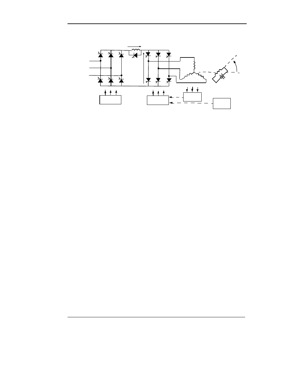
The basic thyristor based load-commutated inverter synchronous motor drive
system is shown in Figure 15.7. In this drive, two static converter bridges are
connected on their DC side by means of a so-called DC link having only a n
inductor on the DC side. The line side converter ordinarily takes power from a
constant frequency bus and produces a controlled DC voltage at its end of the
DC link inductor. The DC link inductor effectively turns the line side converter
into a current source as seen by the machine side converter. Current flow in the
line side converter is controlled by adjusting the firing angle of the bridge and
by natural commutation of the AC line.
The machine side converter normally operates in the inversion mode. Since
the polarity of the machine voltage must be instantaneously positive as the cur-
rent flows into the motor to commutate the bridge thyristors, the synchronous
machine must operate at a sufficiently leading power factor to provide the volt-
seconds necessary to overcome the internal reactance opposing the transfer of
current from phase to phase (commutating reactance). Such load EMF-depen-
dent commutation is called load commutation. As a result of the action of the
10
AC Motor Speed Control
Draft Date: February 5, 2002
link inductor, such an inverter is frequently termed a naturally commutated
current source inverter.
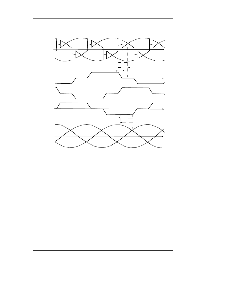
Figure 15.8 illustrates typical circuit operation. Inverter thyristors 1-6 fire
in sequence, one every 60 electrical degrees of operation, and the motor cur-
rents form balanced three-phase quasi-rectangular waves. The electrical angles
shown in Figure 15.8 pertain to commutation from thyristor 1 to 3. The instant
of commutation of this thyristor pair is defined by the phase advance angle
β
relative to the machine terminal voltage V
ab
. Once thyristor 3 is switched on,
the machine voltage V
ab
forces current from phase a to phase b. The rate of rise
of current in thyristor 3 is limited by the commutating reactance, which is
approximately equal to the subtransient reactance of the machine.
During the interval defined by the commutation overlap angle
µ
the current
in thyristor 3 rises to the DC. link current I
dc
while the current in thyristor 1
falls to zero. At this instant, V
ab
appears as a negative voltage across thyristor 1
for a period defined as the commutation margin angle
∆
. The angle
∆
defines,
in effect, the time available to the thyristor to recover its blocking ability
before it must again support forward voltage. The corresponding time T
r
=
∆
/
ω
is called the recovery time of the thyristor. The phase advance angle
β
is equal
to the sum of
µ
plus
∆
. The angle
β
is defined with respect to the motor termi-
nal voltage. In practice it is useful to define a different angle
γ
o
measured with
respect to the internal EMF of the machine. This angle is called the firing
angle. Since the internal EMFs are simply equal to the time rate of change of
the rotor flux linking the stator windings, the firing angle
γ
o
can be located
Figure 15.7
Load commutated inverter synchronous motor drive
Terminal
Voltages
Inverter
Rectifier
Control
Control
Rotor
Position
V
bus
I
dc
θ
γ
0
β
Τ1
Τ3
Τ5
Τ4
Τ6
Τ2
a
b
c
s
Rotor
Stator
AC Supply
Thyristor Based Load-Commutated Inverter Synchronous Motor Drives
11
Draft Date: February 5, 2002
physically as the instantaneous position of the salient poles of the machine, i.e.
the d–axis of the machine relative to the magnetic axis of the outgoing phase
that is undergoing commutation (in case phase a). Hence, in general, the sys-
tem is typically operated in a self-synchronous mode where the output shaft
position (or a derived position-dependent signal) is used to determine the
applied stator frequency and phase angle of current.
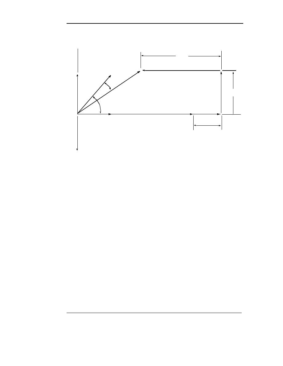
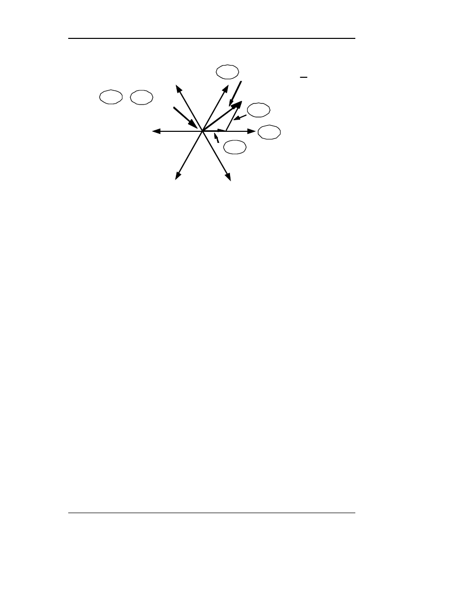
A fundamental component per-phase phasor diagram of Figure 15.9 illus-
trates this requirement. In this figure the electrical angle
γ
is the equivalent of
γ
o
but corresponds to the phase displacement of the fundamental component of
stator current with respect to the EMF. Spatially,
γ
corresponds to 90° minus
the angle between the stator and rotor MMFs and may be called the MMF
Figure 15.8
Load commutated synchronous motor waveforms and control
variables
i
a
i
b
i
c
Thyristor T1
Thyristor T4
Thyristor T3
Thyristor T6
Thyristor T5
Thyristor T2
e
c
e
a
e
b
γ
0
µ
β
∆
γ
12
AC Motor Speed Control
Draft Date: February 5, 2002
angle. A large leading MMF angle
γ
is clearly necessary to obtain a leading ter-
minal power factor angle
φ
.
15.3.1
Torque Production in a Load Commutated Inverter
Synchronous Motor Drive
The average torque developed by the machine is related to the power deliv-
ered to the internal EMF E
i
and, from Figure 15.9, can be written as:
(15.9)
where
ω
rm
is the mechanical speed (i.e.
ω
rm
= 2
ω
e
/P for steady state condi-
tions). The angle
γ
is the electrical angle between the internal EMF and the
fundamental component of the corresponding phase current and is located in
Figure 15.8 for the c phase. It should be noted that this angle is very close the
angle
γ
0
which corresponds to a physical angle which can be set by means of a
suitably located position sensor.
In general, E
i
is speed-dependent,
(15.10)
Figure 15.9
Phasor diagram for load commutated inverter synchronous
motor drive
d-axis
I
d
I
s
I
q
V
s
x
d
I
d
x
q
I
q
E
q
E
i
q-axis
γ
φ
(
x
d
- x
q
)I
d
T
e
3E
i
I
s
γ
cos
ω
rm
------------------------
=
E
i
P
2
---
ω
rm
λ
af
=

Thyristor Based Load-Commutated Inverter Synchronous Motor Drives
13
Draft Date: February 5, 2002
and the apparent speed dependence vanishes whereupon Equation (15.9) takes
the form,
(15.11)
where
λ
af
is rms value of the field flux linking a stator phase winding. Thus,
for a fixed value of the internal angle
γ
, the system behaves very much like a
DC machine and its steady state torque control principles are possible.
15.3.2
Torque Capability Curves
One useful measure of drive performance is a curve showing the maximum
torque available over its entire speed range. A synchronous motor supplied
from a variable-voltage, variable-frequency supply will exhibit a torque-speed
characteristic similar to that of a DC shunt motor. If field excitation control is
provided, operation above base speed in a field-weakened mode is possible and
is used widely. The upper speed limit is dictated by the required commutation
margin time of the inverter thyristors.
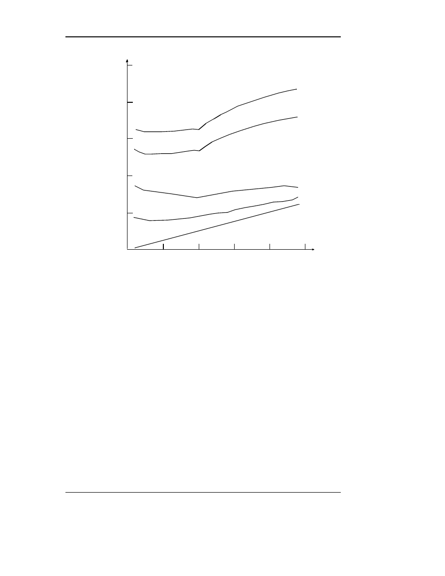
Figure 15.10 is a typical capability curve assuming operation at constant-
rated DC link current, at rated (maximum) converter DC voltage above rated
speed and with a commutation margin time
∆
/
ω
o
of 26.5 ms corresponding to
∆
= 12° at 50 Hz. At very low speeds, where the commutation time is of the
order of the motor transient time constants, the machine resistances make up a
significant part of the commutation impedance. The firing angle must subse-
quently be increased to provide sufficient volt-seconds for commutation as
shown by the companion curves of Figure 15.11. The resulting increase in
internal power factor angle reduces the torque capability. At intermediate
speeds the margin angle can be reduced to values less than 12° to maintain 26.5
ms margin time and slightly greater than rated torque can be produced.
Above rated speed the inverter voltage is maintained constant and the
drive, in effect, operates in the constant kilovolt-ampere mode. The DC
inverter voltage reaches the maximum value allowed by the device ratings and
the maximum output of the rectifier. Although Figure 15.10 shows a weaken-
ing of the field in the high-speed condition, the reduction is not as great as the
inverse speed relationship required for constant horsepower operation. This
again is a consequence of the constant commutation margin angle control.
Since the margin angle increases with speed, i.e. frequency, to maintain the
same margin time, the corresponding increase in power factor angle results in a
T
e
3
2
--- P
λ
af
I
s
γ
cos
=
14
AC Motor Speed Control
Draft Date: February 5, 2002
greater demagnetizing component of stator MMF This offsets partly the need
to weaken the field in the high-speed region.
15.3.3
Constant Speed Performance
When the DC link current is limited to its rated value, the maximum torque can
be obtained from the capability curve (Figure 15.10). However, operation
below maximum torque requires a reduction in the DC link current. When the
field current is adjusted to keep the margin angle
∆
at its limiting value, the
curves of Figure 15.12 result. It can be noted that the torque is now essentially
a linear function of DC link current so that the DC link current command
becomes, in effect, the torque command.
Figure 15.10
Capability curve of a load commutated inverter
synchronous motor drive with constant DC link current and
fixed commutation margin time, field weakening operation
above one p.u. speed assumes operation at constant DC link
voltage
V
dc
T
e
I
f
V
dc
T
e
I
f
To
rq
u
e
(P
er
U
n
it
)
Speed (Per Unit)
0.00
0.20
0.40
0.60
0.80
1.00
1.20
0.00
0.50
1.00
1.50
2.00
2.50
Thyristor Based Load-Commutated Inverter Synchronous Motor Drives
15
Draft Date: February 5, 2002
15.3.4
Control Considerations
Direct control of
γ
0
by use of a rotor position sensor has traditionally been
applied in load commutated inverter drives but has largely been replaced by
schemes using terminal voltage and current sensing to indirectly control
γ
. the
basic principle is to use Eq. (15.11) as the control equation. If terminal voltage
across the machine and the dc link current are measured, then if
γ
is held con-
stant the dc link current required for given torque is
(15.12)
The dc link current that must be supplied can be determined from the current Is
by relating the fundamental component of a quasi-rectangular motor phase cur-
Figure 15.11
Characteristic electrical control angles for load commutated
synchronous motor drive
γ
0
γ
µ
φ
δ
0
20
40
60
80
100
0.00
0.50
1.00
1.50
2.00
2.50
D
e
g
re
e
s
Speed (Per Unit)
I
s
T
e
ω
rm
3E
i
γ
cos
--------------------
=
16
AC Motor Speed Control
Draft Date: February 5, 2002
rent (see Figure 15.8) to its peak value I
dc
. The result is, with reasonable
approximation
(15.13)
The internal rms phase voltage E
i
can be calculated by considering the reactive
drop and is obtained from Figure 15.9. Control is implemented such that the
machine side converter is controlled to maintain either
γ
or
β
constant while
the line side converter is controlled to provide the correct dc link current to sat-
isfy Eq. (15.12) [
Direct control of the commutation margin angle
∆
(more correctly, the mar-
gin time
∆
/
ω
o
where
ω
o
is the motor angular frequency) has the advantage of
causing operation at the highest possible power factor and hence gives the best
utilization of the machine windings. The waveforms in Figure 15.11 also dem-
onstrate that changes in the commutation overlap angle
µ
resulting from cur-
rent or speed changes produce significant differences between the actual value
of
γ
and the ideal value
γ
o
. For this reason, compensators are required in direct
Figure 15.12 DC field current required to produce a linear variation of
Torque with DC link current, operation at rated speed,
margin angle
∆
= 10o
C
u
rr
e
n
t
o
r
To
rq
u
e
(
P
er
U
n
it
)
DC Link Current (Per Unit)
0.00
0.40
0.80
1.20
1.60
0.00
0.40
0.80
1.20
1.60
Te
If
I
dc
π
6
------- I
s
=
Transistor Based Variable-Frequency Induction Motor Drives
17
Draft Date: February 5, 2002
γ
controllers. This compensation is automatic in systems based on controlling
the margin angle
∆
.
15.4 Transistor Based Variable-Frequency Induction
Motor Drives
15.4.1
Introduction
Variable-frequency AC drives are now available from fractional kilowatts to
very large sizes, e.g. to 15 000 kW for use in electric generating stations. In
large sizes, naturally commutated converters are more common, usually driv-
ing synchronous motors. However, in low to medium sizes (up to approxi-
mately 750kW) transistor based PWM voltage source converters driving
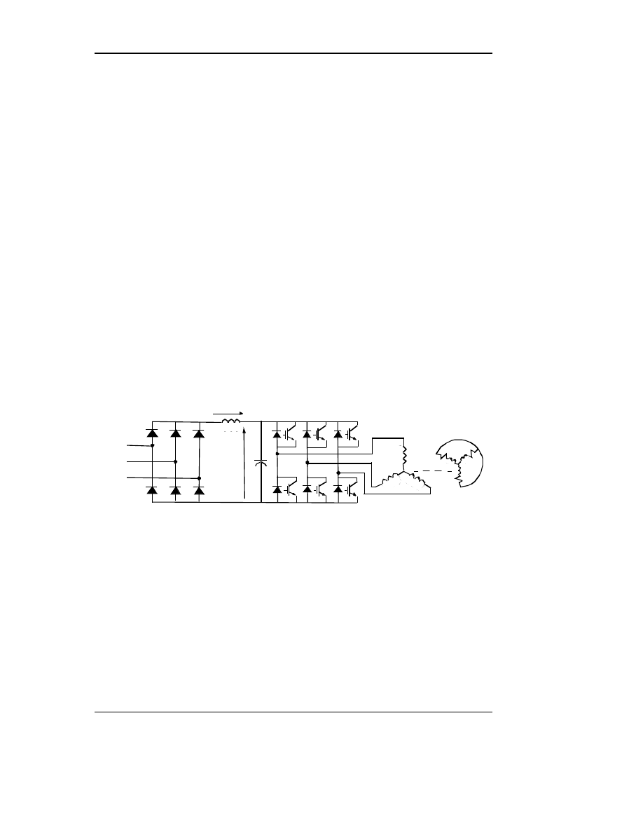
induction motors are almost exclusively used. Figure 15.13 illustrates the basic
power circuit topology of the voltage source inverter. Only the main power-
handling devices are shown; auxiliary circuitry such as snubbers or commuta-
tion elements are excluded.
The modern strategy for controlling the AC output of such a power electronic
converters is the technique known as Pulse-Width Modulation (PWM), which
varies the duty cycle (or mark-space ratio) of the converter switch(es) at a high
switching frequency to achieve a target average low frequency output voltage
or current. In principle, all modulation schemes aim to create trains of switched
pulses which have the same fundamental volt–second average (i.e. the integral
of the waveform over time) as a target reference waveform at any instant. The
Figure 15.13 Basic circuit topology of pulse-width modulated inverter
drive
V
bus
I
dc
Τ1
Τ3
Τ5
Τ4
Τ6
Τ2
a
b
c
s
Stator
AC
Supply
Induction Motor
Pulse-Width Modulated Inverter
Diode Rectifier
Link Filter

18
AC Motor Speed Control
Draft Date: February 5, 2002
major difficulty with these trains of switched pulses is that they also contain
unwanted harmonic components which should be minimized.
Three main techniques for PWM exist. These alternatives are:
1. switching at the intersection of a target reference waveform and a high
frequency triangular carrier (Double Edged Naturally Sampled Sine-
Triangle PWM).
2. switching at the intersection between a regularly sampled reference
waveform and a high frequency triangular carrier (Double Edged Regu-
lar Sampled Sine-Triangle PWM)).
3. switching so that the amplitude and phase of the target reference
expressed as a vector is the same as the integrated area of the converter
switched output over the carrier interval (Space Vector PWM).
Many variations of these three alternatives have been published, and it
sometimes can be quite difficult to see their underlying commonality. For
example, the space vector modulation strategy, which is often claimed to be a
completely different approach to modulation, is really only a variation of regu-
lar sampled PWM which specifies the same switched pulse widths but only
places them a little differently in each carrier interval.
15.4.2
Double Edged Naturally Sampled Sine-Triangle PWM
The most common form of PWM is the naturally sampled method in which a
sine wave command is compared with a high frequency triangle as shown for
one of three phases in Figure 15.14. Intersections of the commanded sine wave
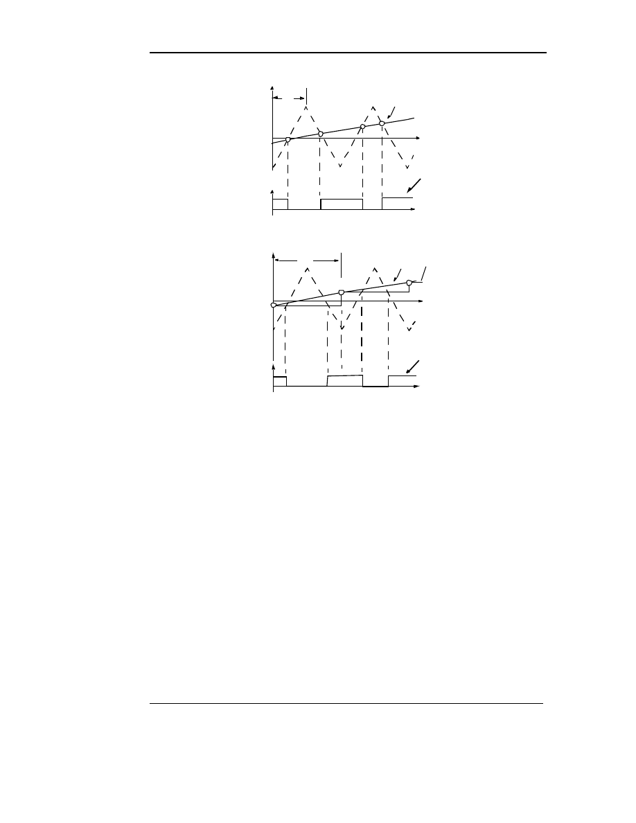
and the triangle produce switching in the inverter as shown in Figure 15.15.
The triangle wave is common to all three phases. Figure 15.15(b) shows the
modulation process in detail, expanded over a time interval of two subcycles,
∆
Τ
/2
. Note that because of switching action the potentials of all three phases
are all equal making the three line to line voltages (and thus the motor phase
voltages) zero. The width of these zero voltage intervals essentially provides
the means to vary the fundamental component of voltage when the frequency
is adjusted so as to realize constant volts/Hz (nearly constant stator flux) oper-
ation. A close inspection of Figure 15.14 indicates that this method does not
fully utilize the available DC voltage since the sine wave command amplitude
reaches the peak of the triangle wave only when the output line voltage is 2/
π
or 0.785 of the maximum possible value of . This deficiency can be
V
b u s
Transistor Based Variable-Frequency Induction Motor Drives
19
Draft Date: February 5, 2002
reduced by introducing a zero sequence third harmonic component command
into each of the controllers. With a third harmonic amplitude of 1/6 that of the
sine wave command, the output can be shown to be increased to or
0.866V
bus
. Additional zero sequence harmonics can be introduced to further
increase the output to or 0.907V
bus
. Further increases in voltage can
only be obtained by introducing low frequency odd harmonic into the output
waveform.
15.4.3
Double Edged Regular Sampled Sine-Triangle PWM
One major limitation with naturally sampled PWM is the difficulty of its
implementation in a digital modulation system, because the intersection
between the reference sinusoid and the triangular or saw-tooth carrier is
defined by a transcendental equation and is complex to calculate. To overcome
this limitation the modern alternative is to implement the modulation system
using a “regular sampled” PWM strategy, where the low frequency reference
waveforms are sampled and then held constant during each carrier interval.
These sampled values are then compared against the triangular carrier wave-
form to control the switching process of each phase leg, instead of the sinusoi-
dally varying reference.
The sampled reference waveform must change value at either the positive
or positive/negative peaks of the carrier waveform, depending on the sampling
strategy. This change is required to avoid instantaneously changing the refer-
ence during the ramping period of the carrier, which may cause multiple switch
Figure 15.14 Control principle of naturally sampled PWM showing one of
three phase legs
Vdc
+
-
T
1
T
2
D
1
D
2
Vdc
+
-
Load
+
-
M cos( ot)
+
-
1.0
-1.0
t
vtr
Phase
Leg
a
n
z
p
ω
3
(
)
2
⁄
3
π
(
)
6
⁄
20
AC Motor Speed Control
Draft Date: February 5, 2002
transitions if it was allowed to occur. For a triangular carrier, sampling can be
symmetrical, where the sampled reference is taken at either the positive or neg-
ative peak of the carrier and held constant for the entire carrier interval, or
asymmetrical, where the reference is re-sampled every half carrier interval at
both the positive and the negative carrier peak. The asymmetrical sampling is
preferred since the update rate of the sampled waveform is doubled resulting in
a doubling in the harmonic spectrum resulting from the PWM process. The
phase delay in the sampled waveform can be corrected by phase advancing the
reference waveform.
Figure 15.15
(a) Naturally sampled PWM and (b) symmetrically sampled
PWM
0
0
0
0
(a)
(b)
t
t
∆
T
v
as
*
v
as
*
(sampled)
v
an
∆
T
v
an
v
a s
*
Transistor Based Variable-Frequency Induction Motor Drives
21
Draft Date: February 5, 2002
15.4.4
Space Vector PWM
In the mid 1980's a form of PWM called “Space Vector Modulation” (SVM)
was proposed, which was claimed to offer significant advantages over natural
and regular sampled PWM in terms of performance, ease of implementation
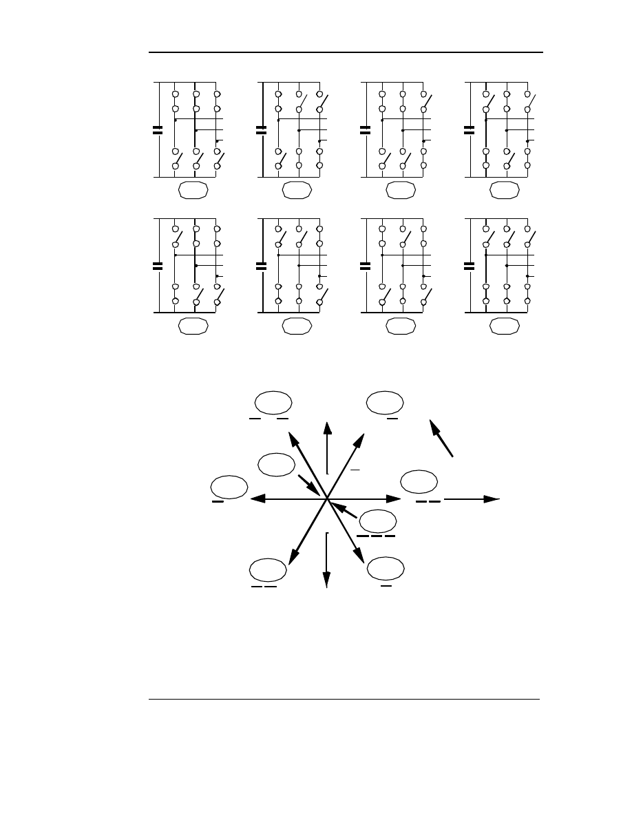
and maximum transfer ratio [4], [5]. The principle of SVM is based on the fact
that there are only 8 possible switch combinations for a three phase inverter.
The basic inverter switch states are shown in Figure 15.17. Two of these states
(SV
0
and SV
7
) correspond to the short circuit discussed previously, while the
other six can be considered to form stationary vectors in the d-q plane as
shown in Figure 15.19. The magnitude of each of the six active vectors is,
(15.14)
corresponding to the maximum possible phase voltage. Having identified the
stationary vectors, at any point in time, an arbitrary target output voltage vector
can then be made up by the summation (“averaging”) of the adjacent space
vectors within one switching period , as shown in Figure 15.19 for a target
vector in the first 60
o
segment of the plane. Target vectors in the other five seg-
ments of the hexagon are clearly obtained in a similar manner.
For ease in notation, the d–q plane can be considered as being complex.
The geometric summation shown in Figure 15.19 can then be expressed math-
ematically as
(15.15)
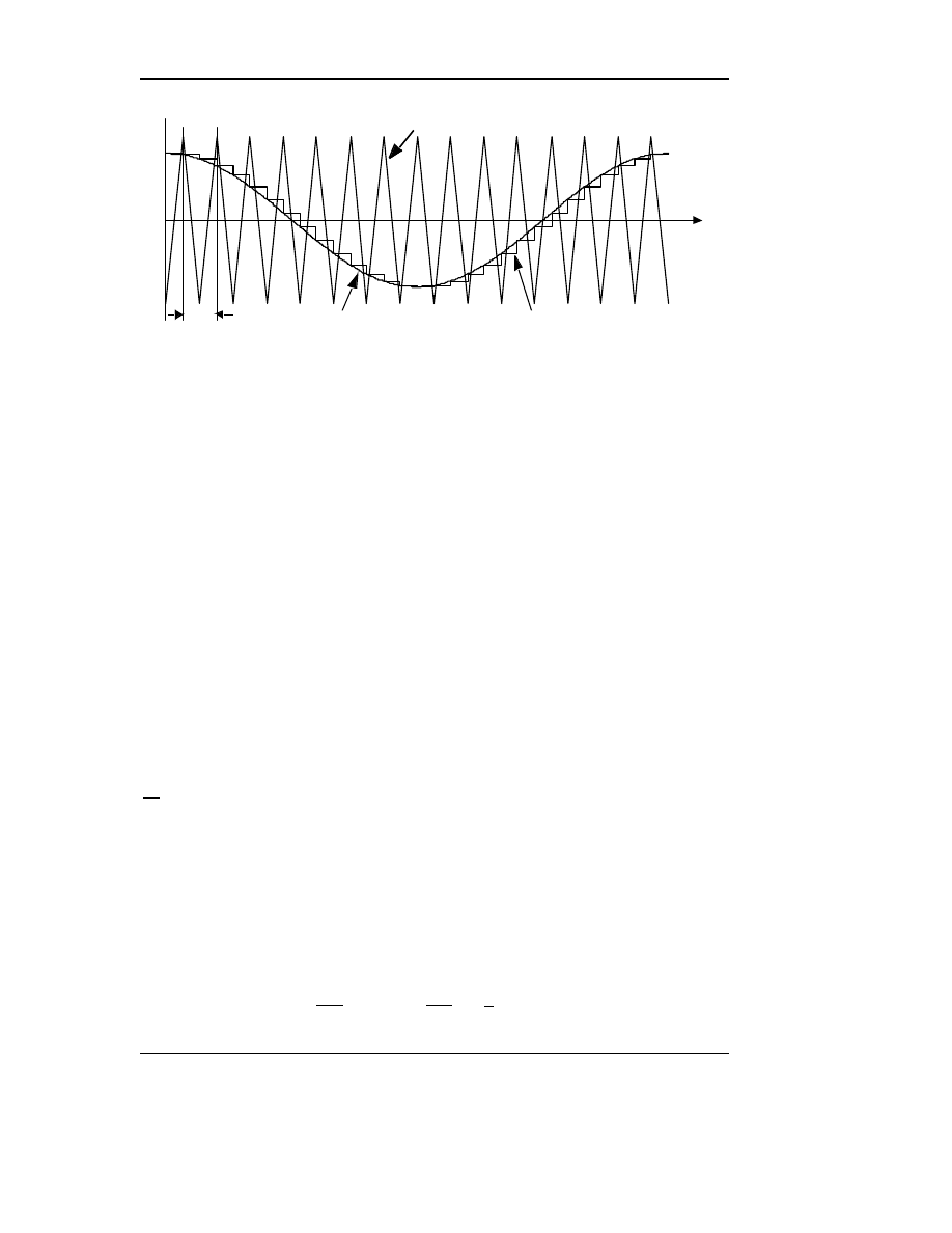
Triangular Carrier
Asymmetrically Sampled Reference
Sinusoidal Reference
∆
T
t
Figure 15.16
Regular asymmetrically sampled pulse width modulation
V
m
2
3
--- V
bus
=
V
o
T
∆
T
SV1
T
∆
2
⁄
(
)
------------------SV
1
T
SV2
T
∆
2
⁄
(
)
------------------SV
2
+
V
o
=
22
AC Motor Speed Control
Draft Date: February 5, 2002
Figure 15.17 Eight possible phase leg switch combinations for a VSI
SV
1
SV
0
SV
2
SV
3
SV
5
SV
4
SV
6
SV
7
a
b
c
a
a
a
a
a
a
a
b
b
b
b
b
b
b
c
c
c
c
c
c
c
S1
S1
S1
S1
S1
S1
S1
S1
S6
S3
S3
S3
S3
S3
S3
S3
S3
S5
S5
S5
S5
S5
S5
S5
S5
S4
S4
S4
S4
S4
S4
S4
S4
S6
S6
S6
S6
S6
S6
S6
S2
S2
S2
S2
S2
S2
S2
S2
Figure 15.18 Location of the eight possible stationary voltage
vectors for a VSI in the d–q (Re–Im) plane. Each
vector has a length (2/3)V
bus
S
1
.S
3
.S
5
S
1
.S
3
.S
5
S
1
.S
3
.S
5
S
1
.S
3
.S
5
S
1
.S
3
.S
5
S
1
.S
3
.S
5
S
1
.S
3
.S
5
θ
o
Im (–d ) Axis
Re (q ) Axis
d Axis
2
3
V
dc
S
1
.S
3
.S
5
SV1
SV2
SV3
SV5
SV6
SV7
SV0
SV4
Transistor Based Variable-Frequency Induction Motor Drives
23
Draft Date: February 5, 2002
for each switching period of . That is, each active space vector is
selected for some interval of time which is less than the one-half carrier period.
It can be noted that SVM is an intrinsically a regular sampled process, since in
essence it matches the sum of two space vector volt–second averages over a
half carrier period to a sampled target volt–second average over the (15.15)
(15.16)
or in cartesian form:
(15.17)
Equating real and imaginary components yields the solution,
(15.18)
(15.19)
Space Vector V
o
Sampled Target
o
θ
SV2
SV1
SV1
SV2
for time T
sv1
SV7
SV0
+
for time
∆
T/2-T
sv1
-T
sv2
for time T
sv2
Figure 15.19
Creation of an arbitrary output target phasor by the
geometrical summation of the two nearest space vectors
T
∆
2
⁄
T
SV 1
V
m
0
∠
T
SV2
V
m
π
3
⁄
∠
+
T
∆
2
-------
V
o
θ
o
∠
=
T
SV1
V
m
T
SV2
V
m
π
3
---
cos
j
π
3
---
sin
+
+
V
o
θ
o
cos
j
θ
o
sin
+
(
)
T
∆
2
-------
=
T
SV 1
V
o
V
m
-------
π
3
---
θ
o
–
sin
π
3
---
sin
----------------------------
T
∆
2
------- (active time for SV1)
=
T
SV 2
V
o
V
m
-------
θ
o
( )
sin
π
3
---
sin
------------------
T
∆
2
------- (active time for SV2)
=

24
AC Motor Speed Control
Draft Date: February 5, 2002
Since , the maximum possible magnitude for V
o
is V
m
,
which can occur at
.
In addition a further constraint is that the sum of the active times for the
two space vectors obviously cannot exceed the half carrier period, i.e.
. From simple geometry, the limiting case for this occurs
at
, which means,
(15.20)
and this relationship constrains the maximum possible magnitude of V
o
to
(15.21)
Since V
o
is the magnitude of the output phase voltage, the maximum possi-
ble l–l output voltage using SVM must equal:
(15.22)
This result represents an increase of or 1.1547 compared to regular
sampled PWM (Section 15.4.2) but is essentially the same when zero sequence
harmonics are added to the voltage command as was previously discussed.
15.4.5
Constant Volts/Hertz Induction Motor Drives
The operation of induction machines in a constant volts per hertz mode back to
the late fifties and early sixties but were limited in their low speed range[6].
Today constant volt per hertz drives are built using PWM-IGBT-based invert-
ers of the types discussed in Sections 15.4.2 to 15.4.4 and the speed range has
widened to include very low speeds [7] although operation very near zero
speed (less than 1 Hz) remains as a challenge mainly due to inverter non-lin-
earities at low output voltages.
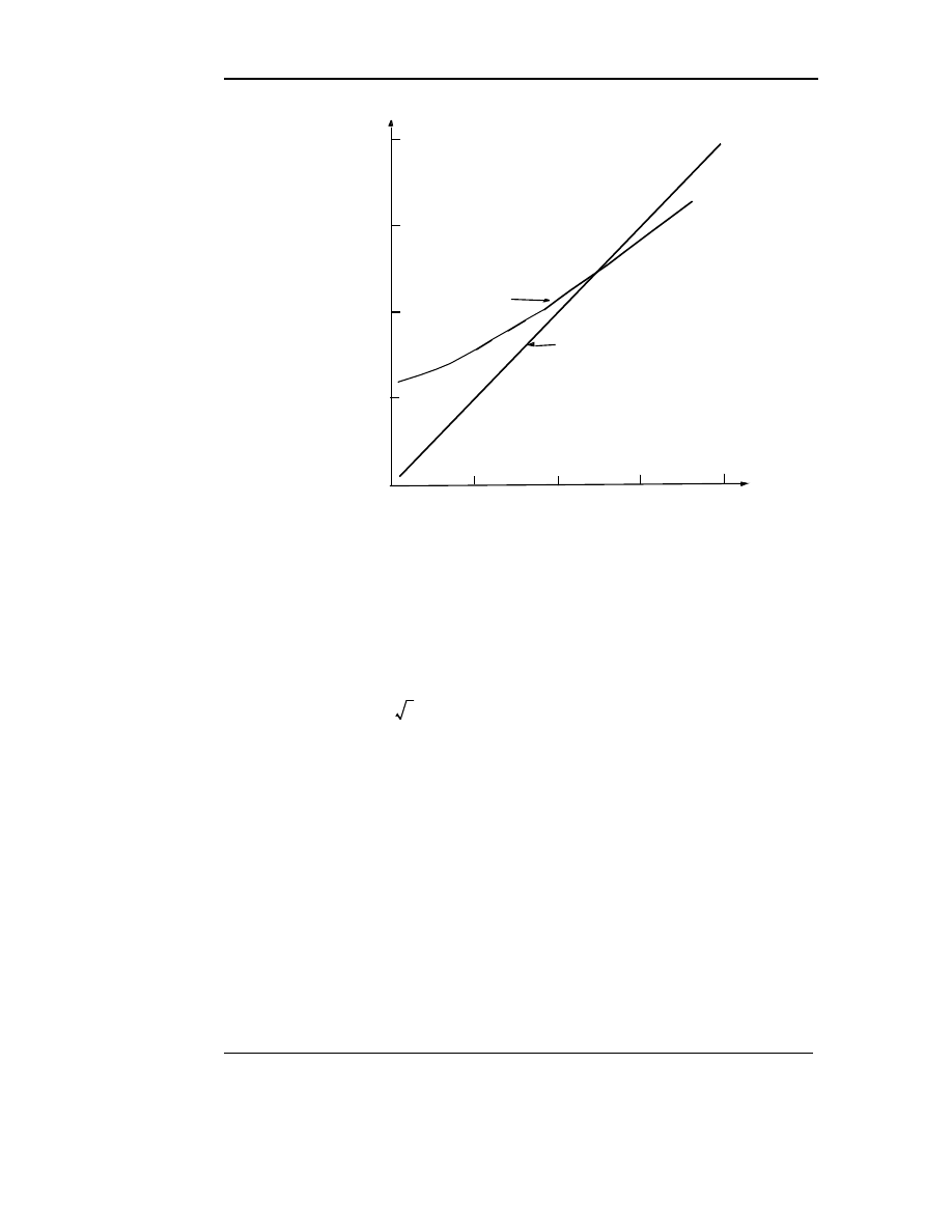
Ideally, by keeping a constant V/f ratio for all frequencies the nominal
torque-speed curve of the induction motor can be reproduced at any frequency
as discussed in Section 15.2.2. Specifically if stator resistance is neglected and
keeping a constant slip frequency the steady state behavior of the induction
machine can be characterized as an impedance proportional to frequency.
Therefore, if the V/f ratio is kept constant the stator flux, stator current, and
0
T
SV1
≤
T
SV2
T
∆
2
⁄
≤
,
θ
o
0
°
or
π
3
⁄
=
T
SV 1
T
SV2
+
T 2
⁄
∆
≤
θ
o
π
6
⁄
=
T
SV 1
T
SV2
+
T
∆
2
-------
-----------------------------
V
o
V
m
-------
2
π
6
---
sin
π
3
---
sin
--------------
1
≤
=
V
o
V
m
π
3
---
sin
1
3
------- V
bus
=
=
V
o l
l
–
(
)
3V
o
V
bus
=
=
2
3
(
)
⁄

Transistor Based Variable-Frequency Induction Motor Drives
25
Draft Date: February 5, 2002
torque will be constant at any frequency. This feature suggests that to control
the torque one needs to simply apply the correct amount of V/Hz to stator
windings. This simple, straight forward approach, however, does not work well
in reality due to several factors, the most important ones being
1) Effect of supply voltage variations
2) Influence of stator resistance
3) Non-ideal torque/speed characteristic (effects of slip)
4) Non-linearities introduced by the PWM inverter.
Low frequency operation is the particularly difficult to achieve since these
effects are most important at low voltages. Also, the non-linearities within the
inverter, if not adequately compensated, yield highly distorted output voltages
which, in turn, produces pulsating torques that lead to vibrations and increased
acoustic noise.
In addition to these considerations, a general purpose inverter must accom-
modate a variety of motors from different manufacturers. Hence it must com-
pensate for the above mentioned effects regardless of machine parameters. The
control strategy must also be capable of handling parameter variations due to
temperature and/or saturation effects. This fact indicates that in a true “general
purpose” inverter it is necessary to include some means to estimate and/or
measure some of the machine parameters. Another aspect that must be consid-
ered in any practical implementation deals with the DC bus voltage regulation,
which, if not taken into account, may lead to large errors in the output voltage.
Because general purpose drives are cost sensitive it is also desired to
reduce the number of sensing devices within the inverter. Generally speaking
only the do link inverter voltage and current are measured, hence the stator cur-
rent and voltage must be estimated based only on these measurements. Speed
encoders or tachometers are not used because they add cost as well as reduce
system reliability.
Other aspects that must be considered in the implementation of an “ideal
constant V/f drive” relate to:
a) current measurement and regulation,
b) changes in gain due to pulse dropping in the PWM inverter,

26
AC Motor Speed Control
Draft Date: February 5, 2002
c) instabilities due to poor volt-second compensation that result in lower
damping. This problem is more important in high efficiency motors, and
d) quantization effects in the measured variables.
Another aspect that must be carefully taken into account is the quantization
effect introduced by the A/D converters used for signal acquisition. A good
cost to resolution compromise seems to be the use of 10 bit converters. How-
ever, a high performance drive is likely to require 12 bit accuracy.
15.4.6
Required Performance of Control Algorithms
The key features of a typical control algorithm, is defined as follows:
a) Open loop speed accuracy: 0.3-0.5% (5.4 to 8.2 rpm)
b) Speed control region: 1-30 to 1:50 (60 - 1.2 Hz to 60 - 2 Hz)
c) Torque range: 0 to 150%
c) Output voltage accuracy: 1-2% (1.15 - 2.3 volts)
d) Speed response with respect to load changes: less than 2 seconds
e) Self commissioning capabilities: parameter estimation error less than
10%
f) Torque-slip linearity: within 10-15%
g) Energy saving mode: for no-load operation the power consumed by the
motor must be reduced by 20% with respect to the power consumed at full
flux and no load.
Current sensors are normally of the open-loop type and their output needs
to be compensated for offset and linearity. In addition the DC link bus voltage
is typically measured. The switching frequency for the PWM is fixed at typi-
cally 10 to 12 kHz.
It is frequently also required to measure or estimate the machine parame-
ters used to implement the control algorithms. In such cases it is assumed that
the number of poles, rated power, rated voltage, rated current, and rated fre-
quency are known.
15.4.7
Compensation for Supply Voltage Variations
In an industrial environment, a motor drive is frequently subjected to supply
voltage fluctuations which, in turn, imposed voltage fluctuations on the DC

Transistor Based Variable-Frequency Induction Motor Drives
27
Draft Date: February 5, 2002
link of the inverter. If these variations are not compensated for, the motor will
be impressed with either and under or an overvoltage which produces exces-
sive I
2
r loss or excessive iron loss respectively. The problem can be avoided if
the DC link voltage is measured and the voltage command adjusted to
produce a modified command such that
(15.23)
where is the rated value of bus voltage.
15.4.8
Ir Compensation
A simple means to compensate for the resistive drop is to boost the stator volt-
age by I
1
*r
1
(voltage proportional to the current magnitude) and neglect the
effect of the current phase angle. To avoid the direct measurement of the stator
current this quantity can be estimated from the magnitude of the dc-link cur-
rent [8]. In this paper a good ac current estimate was demonstrated at frequen-
cies as low as 2 Hz but the system requires high accuracy in the dc-link current
measurement making it impractical for low cost applications. A robust Ir boost
method must include both magnitude and phase angle compensation. Typically
currents of two phases must be measured with the third current inferred since
the currents sum to zero. In either case the value of the stator resistance must
be known.
The value of the stator resistance can be estimated by using any one of sev-
eral known techniques [9]–[11]. Unfortunately these parameter estimation
techniques require knowing the rotor position or velocity and the stator current.
An alternate method of `boosting' the stator voltage at low frequencies is pre-
sented in [12]. Here the V/f ratio is adjusted by using the change in the sine of
the phase angle of motor impedance. This approach also requires knowing the
rotor speed and it is also dependent on the variation of the other machine
parameters. Its practical usefulness is questionable because of the technical dif-
ficulty of measuring phase angles at frequencies below 2 Hz.
Constant Volts/Hz control strategy is typically based on keeping the stator
flux-linkage magnitude constant and equal to its rated value. Using the steady
state equivalent circuit of the induction motor, shown in Figure 15.3, an
expression for stator voltage compensation for resistive drop can be shown to
be
V
1
∗
V
1
∗∗
V
1
∗∗
V
busR
V
b u s
-------------
V
1
∗
=
V
busR
28
AC Motor Speed Control
Draft Date: February 5, 2002
(15.24)
where is the base (rated) rms phase voltage at base frequency, is the
rated frequency in Hertz, is the estimated value of resistance, is the rms
current obtained on a instantaneous basis by,
(15.25)
and is the real component of rms stator current obtained from
(15.26)
where and are two of the instantaneous three phase stator currents
and the cosine terms are obtained from the voltage command sig-
nals. The estimated value of resistance can be obtained either by a simple dc
current measurement corrected for temperature rise or by a variety of known
methods[13]–[15]. Derivation details of these equations are found in [16].
Given the inherently positive feedback characteristic of an Ir boost algorithm it
is necessary to stabilize the system by introducing a first order lag in the feed-
back loop (low-pass filter).
15.4.9
Slip Compensation
By its nature, the induction motor develops its torque as a rotor speed slightly
lower than synchronous speed (effects of slip). In order to achieve a desired
speed, the applied frequency must therefore be increased by an amount equal
to the slip frequency. The usual method of correction is to assume a linear rela-
tionship exists between torque and speed in the range of interest, Hence, the
slip can be compensated by knowing this relationship. This approximation
gives good results as long as the breakdown torque is not approached. How-
ever, for high loads the relationship becomes non-linear. Ref. [16] describes a
correction which can be used for high slip,
V
1
2
3
------- I
1 Re
( )
R
ˆ
1
⋅
V
1R
f
e
f
R
-------------
2
9
--- i
1 r e
( )
R
ˆ
1
⋅
(
)
2
I
1
R
ˆ
1
(
)
2
–
+
+
=
V
1R
f
R
Rˆ
1
I
s
I
s
2
3
--- i
a
i
a
i
c
+
(
)
i
c
2
+
=
I
1 Re
( )
I
1 Re
( )
i
a
θ
e
cos
θ
e
2
π
3
---
–
cos
–
i
c
θ
e
2
π
3
---
+
cos
θ
e
2
π
3
---
–
cos
–
+
=
i
a
i
c
θ
e
ω
e
t
=

Transistor Based Variable-Frequency Induction Motor Drives
29
Draft Date: February 5, 2002
(15.27)
where is the external command frequency and,
(15.28)
and
(15.29)
and P is the number of poles. The slope of the linear portion of the torque–
speed curve is given by
(15.30)
Finally the air gap power is
(15.31)
where at rated frequency can be obtained from
(15.32)
where the caret “^” denotes an estimate of the quantity. The quantities
and are the rated values of slip frequency, line fre-
quency, efficiency, stator current, input power and torque respectively. All of
these quantities can be inferred from the nameplate data.
15.4.10 Volt-Second Compensation
One of the main problems in open-loop controlled PWM-VSI drives is the
non-linearity caused by the non-ideal characteristics of the power switches.
The most important non-linearity is introduced by the necessary blanking time
to avoid short circuiting the DC link during the commutations. To guarantee
that both switches are never on simultaneously a small time delay is added to
f
slip
1
2
A P
gap
⋅
–
----------------------------
f
e
∗
( )
2
S
m
S
R
------ S
linear
2
T
bd
T
R
--------
---------------------- P
gap
⋅
B P
gap
2
⋅
–
+
f
e
∗
–
=
f
e
∗
A
P
4
π
S
bd
T
bd
f
R
----------------------------
=
B
P
4
π
T
bd
---------------
2
=
S
linear
P
π
---
S
R
f
R
T
R
----------
=
P
gap
3V
1
I
1
pf
( )
3I
1
2
R
ˆ
1
P
core
–
–
=
P
c o r e
P
coreR
P
inR
1
η
R
1
S
R
–
--------------
–
3I
1R
2
Rˆ
1
–
=
S
R
f
R
η
R
I
1R
P
inR
, ,
,
,
T
R

30
AC Motor Speed Control
Draft Date: February 5, 2002
the gate signal of the turning-on device. This delay, added to the device's inher-
ent turn-on and turn-off delay times, introduces a magnitude and phase error in
the output voltage[17]. Since the delay is added in every PWM carrier cycle
the magnitude of the error grows in proportion to the switching frequency,
introducing large errors when the switching frequency is high and the total out-
put voltage is small.
The second main non-linear effect is due to the finite voltage drop across
the switch during the on-state[18]. This introduces an additional error in the
magnitude of the output voltage, although somewhat smaller, which needs to
be compensated.
To compensate for the dead-time in the inverter it is necessary to know the
direction of the current and then change the reference voltage by adding or
subtracting the required volt–seconds. Although in principle this is simple, the
dead time also depends on the magnitude and phase of the current and the type
of device used in the inverter. The dead-time introduced by the inverter causes
serious waveform distortion and fundamental voltage drop when the switching
frequency is high compared to the fundamental output frequency. Several
papers have been written on techniques to compensate for the dead
time[17],[19]-[21].
Regardless of the method used, all dead time compensation techniques are
based on the polarity of the current, hence current detection becomes an impor-
tant issue. This is specially true around the zero-crossings where an accurate
measurement is needed to correctly compensate for the dead time. Current
detection becomes more difficult due to the PWM noise and because the use of
filters introduces phase delays that needed to be taken into account.
The name “dead-time compensation” often misleads since the actual dead
time, which is intentionally introduced, is only one of the elements accounting
for the error in the output voltage, for this reason here it is referred as volt-sec-
ond compensation. The volt-second compensation algorithm developed is
based on the average voltage method. Although this technique is not the most
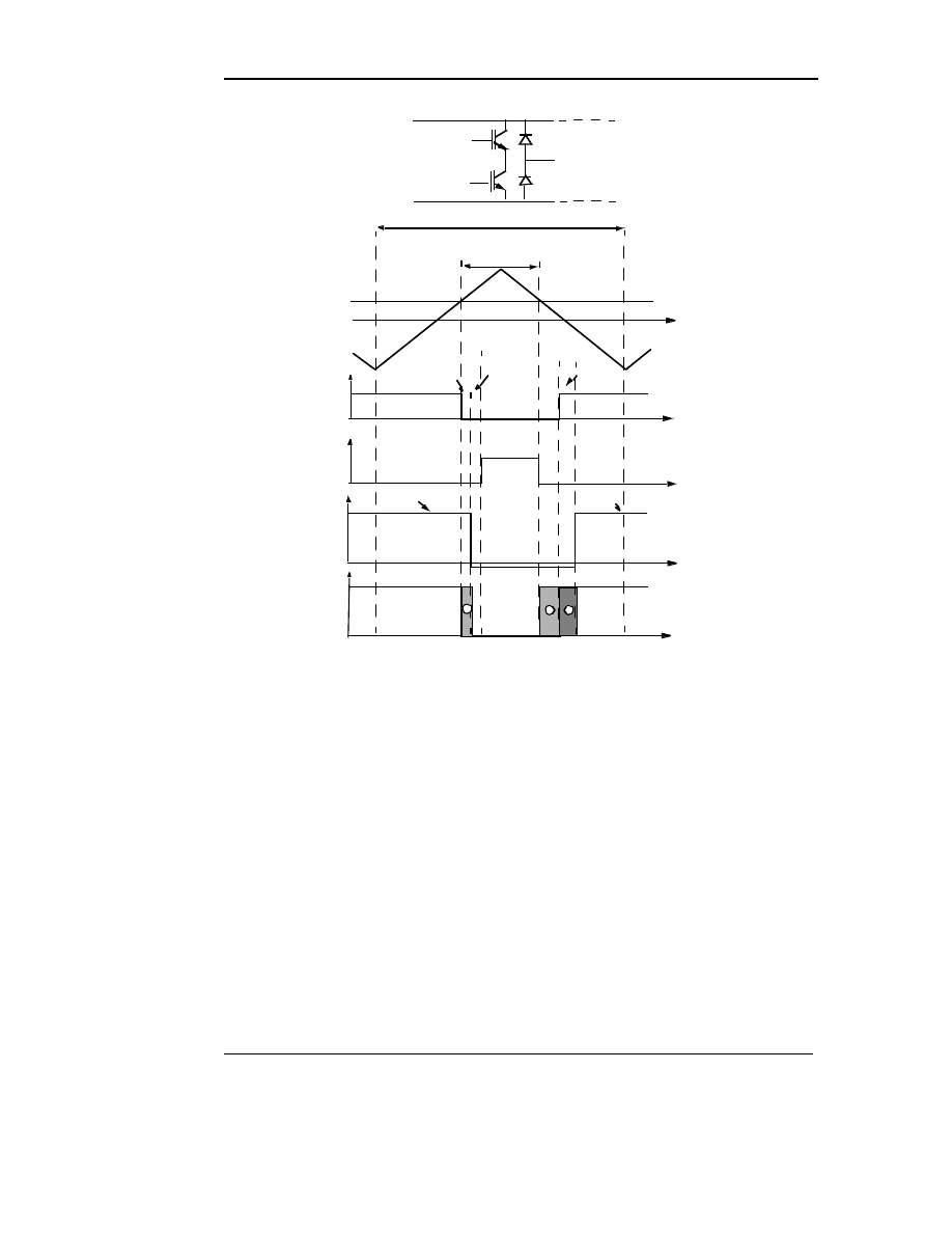
accurate method available it gives good results for steady state operation. Fig-
ure 15.20 shows idealized waveforms of the triangular and reference voltages
over one carrier period. It also shows the gate signals, ideal output voltage, and
pole voltage for positive current. For this condition, the average pole voltage
over one period can be expressed by:

Transistor Based Variable-Frequency Induction Motor Drives
31
Draft Date: February 5, 2002
(15.33)
where:
: average output phase voltage with respect to negative dc bus over
one switching interval,
V
sat
: device saturation voltage,
T
c
: carrier period,
V
bus
: DC link bus voltage,
t
d
: dead time,
t
on
: turn-on delay time,
t
off
: turn-off delay time,
V
d
: diode forward voltage drop..
The first term in Eq. (15.33) represents the ideal output voltage and the
remainder of the terms are the errors caused by the non-ideal behavior of the
inverter. A close examination of the error terms shows that the first and last
terms will be rather large with the middle term being much smaller. Hence one
can approximate the voltage error by
(15.34)
and the output voltage can be expressed as
(15.35)
if the current if positive and
(15.36)
if the current is negative. Since the three motor phase voltage must add to zero
the voltage of phase a with respect to the motor stator neutral s is therefore,
v
an
〈
〉
V
bus
1
2
---
V
∗
θ
cos
V
b u s
-------------------
+
t
d
t
on
t
off
–
+
T
c
----------------------------------
V
bus
V
s a t
V
d
+
–
(
)
–
=
V
s a t
V
d
–
V
bus
------------------------
V
∗
–
V
s a t
V
d
+
2
------------------------
–
v
an
〈
〉
V
∆
t
d
t
on
t
off
–
+
T
c
------------------------------ V
bus
V
sat
–
V
d
+
(
)
V
sat
V
d
+
2
----------------------
+
≈
v
an
V
bus
1
2
---
V
∗
θ
cos
V
b u s
-------------------
+
V
∆
–
≈
v
an
V
bus
1
2
---
V
∗
θ
cos
V
bus
-------------------
+
V
∆
+
≈
32
AC Motor Speed Control
Draft Date: February 5, 2002
(15.37)
The voltages of the remaining two phase voltage are obtain in similar manner.
As shown in Figure 15.20, the voltage error corresponds to the difference
in areas between the commanded voltage and the actual voltage. The (+) and (-
) signs in the bottom trace indicate that in which part of the cycle there is a gain
or loss of voltage. The algebraic sum of these areas gives the average error
over a pulse period. The voltage error can be corrected either on a per pulse
basis or, less accurately, on a per cycle basis. The compensation algorithm is
thus is based on commanding a voltage modified by depending upon the
Figure 15.20
PWM voltage waveforms for positive current
+
–
P
N
a
vaN
vaN*
vg-
vg+
Vbus–Vsat
Vbus–Vsat
–Vd
ton
td
toff
td
–
–
–
+
Vbus
Tc
2
------ 1
2V
∗
V
b u s
-------------
–
T
c
t
t
t
t
t
vg+
vg-
V
1
*
v
as
2
3
--- v
an
1
3
--- v
bn
–
1
3
--- v
cn
–
=
V
∆
±
Field Orientation
33
Draft Date: February 5, 2002
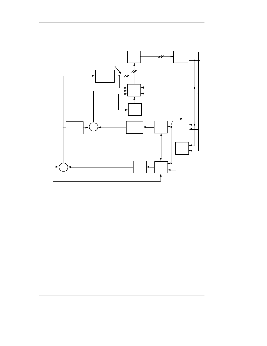
polarity of the current. An overall volts/Hertz control scheme including IR, slip
and volt-second compensation is shown in Figure 15.21[16].
15.5 Field Orientation
15.5.1
Complex Vector Representation of Field Variables
Although the large majority of variable speed applications require only speed
control in which the torque response is only of secondary interest, more chal-
lenging applications such a traction applications, servomotors and the like
depend critically upon the ability of the drive to provide a prescribed torque
whereupon the speed becomes the variable of secondary interest. The method
of torque control in ac machines is called either vector control or, alternatively
Figure 15.21
Complete volts per hertz induction motor speed controller
incorporating IR, slip, DC bus and volt-second compensation
cos(
θ
),cos(
θ
-2
π
/3),cos(
θ
+2
π
/3)
f
e
*
PWM
Inverter
V
bus
∆
V
v
an
,v
bn
,v
cn
v
a s
,v
bs
,v
cs
V
1
**
I
1(Re)
I
1
f
e
**
V
1
*
Eq.
(15.27)
Eq.
(15.31)
Eq.
(15.25)
Eq.
(15.26)
Eq.
(15.24)
Eq.
(15.34)
Eq.
(15.35)
Eq.
(15.37)
1
1
T
fil
s
+
---------------------
s
s2
ω
e
2
+
-------------------
f
ˆ
slip
+
+
+
+
V
1R
f
R
⁄
P
coreR

34
AC Motor Speed Control
Draft Date: February 5, 2002
field orientation. Vector control refers to the manipulation of terminal currents,
flux linkages and voltages to affect the motor torque while field orientation
refers to the manipulation of the field quantities within the motor itself. Since it
is common for machine designers to visualize motor torque production in
terms of the air gap flux densities and MMFs instead of currents and fluxes
which relate to terminal quantities, it is useful to begin first with a discussion
of the relationship between the two viewpoints.
Consider, first of all, the equation describing the instantaneous position of the
stator air gap MMF for a simple two pole. If phase as is sinusoidally distrib-
uted then the MMF in the gap resulting from current flowing in phase a is
.
(15.38)
where is the effective number of turns and
β
is the angle measured in the
counterclockwise direction from the magnetic axis of phase as. Similarly, if
currents flow in phases bs or cs which are spatially displaced from phase as by
120 electrical degrees, then the respective air gap MMFs are:
(15.39)
(15.40)
As written Eqs. (15.38) to (15.40) are real quantities. They would be more
physically insightful if these equations were given spatial properties such that
their maximum values were directed along their magnetic axes which are
clearly spatially oriented with respect to the magnetic axis of phase as.
The can be done by introducing a complex plane in which the unit amplitude
operator provides the necessary spatial orientation. Specifically
spatial quantities and can now be defined where
(15.41)
(15.42)
where † denotes the complex conjugate.
F
a s
N
s
2
----- i
a s
β
cos
=
0
β
2
π
≤ ≤
N
s
F
b s
N
s
2
----- i
b s
β
2
π
3
------
–
cos
=
F
cs
N
s
2
-----i
cs
β
2
π
3
------
+
cos
=
120
°
±
a
e
j2
π
3
⁄
=
F
b s
F
cs
F
b s
aF
b s
a
N
s
2
----- i
b s
β
2
π
3
------
–
cos
=
=
F
cs
a
2
F
cs
a
†
N
s
2
----- i
b s
β
2
π
3
------
–
cos
=
=

Field Orientation
35
Draft Date: February 5, 2002
The net (total) stator air gap MMF expressed as a space vector is simply the
sum of the three components or
(15.43)
Introducing the Euler equation
(15.44)
Eq. (15.43) can be manipulated to the form
(15.45)
where, if the three phase current sum to zero,
(15.46)
(15.47)
Eq. (15.45) is general in the sense that the three stator currents are arbitrary
functions of time (but must sum to zero). Consider now the special case when
the currents are balanced and sinusoidal. In this case it can be shown that
(15.48)
and
where I is the amplitude of each of the phase currents and . The corre-
sponding MMF is
(15.49)
The stator current in complex form can be clearly visualized as a “vec-
tor” having a length I
s
making an angle
θ
with respect to the real axis. On the
other hand, the complex MMF quantity is not strictly a vector since it
has spatial as well has temporal attributes. In particular varies as a sinu-
soidal function of the spatial variable
β
. However at a particular time instant
the maximum positive value of the MMF is, from (15.49), clearly
located spatially at . Hence, the temporal (time) position of the current
vector also locates the instantaneous spatial position of the corresponding
MMF amplitude. This basic tenet is essential for the understanding of AC
motor control.
F
abcs
F
a s
aF
bs
a
2
F
cs
+
+
=
e
j
β
β
cos
j
β
sin
+
=
F
abcs
3
2
---
N
s
2
-----
i
abcs
e
j
β
–
i
abcs
†
e
j
β
+
(
)
=
i
abcs
i
a s
ai
bs
a
2
i
cs
+
+
=
i
a s
j
1
3
------- i
b s
i
cs
–
(
)
+
=
i
abcs
Ie
j
θ
=
i
abcs
†
0
=
θ
ω
t
=
F
abcs
3
2
---
N
s
2
-----
I
s
e
j
θ β
–
(
)
=
i
abcs
F
abcs
F
abcs
t
θ ω
⁄
=
β
θ
=

36
AC Motor Speed Control
Draft Date: February 5, 2002
It can be further shown that the temporal position of the air gap flux link-
age can be related to the position of the corresponding flux density by
(15.50)
where is the length of the vector . Thus the location of a flux
linkage vector in the complex plane
γ
uniquely locates the position of the
amplitude of the corresponding flux density along the air gap of the machine.
While not strictly correct in terms of having spatial properties along the air
gap, the flux linkage corresponding to leakage flux is also given an spatial
interpretation in which case, for example, the total rotor flux linkage can be
defined as
(15.51)
where and are the three phase motor stator and rotor currents
treated a complex quantities as in Eq. (15.46).
It should now be clear that while torque production in an AC machine is
physically produced by the interaction (alignment) of the stator MMF relative
to the air gap flux density, it is completely equivalent to view torque produc-
tion as the interaction (alignment) of the stator current vector with respect to
the air gap flux linkage vector. This is the principle of control methods which
concentrates on instantaneous positioning of the stator current vector with
respect to a presumed positioning of the rotor flux vector. The fact that these
temporal based vectors produce spatial positioning of field quantities which
are in simple proportion to these vectors has prompted the use of the term
space vectors for such quantities and the control method termed field orienta-
tion.
15.5.2
The d–q Equations of a Squirrel Cage Induction Motor
Motion control system requirements are typically realized by employing
torque control concepts in the induction machine which are patterned after DC
machine torque control. The action of the commutator of a DC machine in
holding a fixed, orthogonal spatial angle between the field flux density and the
armature MMF is emulated in induction machines by orienting the stator cur-
rent with respect to the rotor flux linkages (i.e the stator MMF with respect to
the rotor flux density as explained above) so as to attain independently con-
B
abc ag
( )
1
2
π
---
τ
p
l
e
N
s
-------------------------
λ
ag
( )
e
j
θ γ
–
(
)
=
λ
ag
( )
λ
a b c a g
( )
λ
abcr
L
2
i
abcr
L
m
i
abcs
i
abcr
+
(
)
+
=
i
abcs
i
abcr

Field Orientation
37
Draft Date: February 5, 2002
trolled flux and torque. Such controllers are called field-oriented controllers
and require independent control of both magnitude and phase of the AC quan-
tities and are, therefore, also referred to as vector controllers. The terms “field
orientation” and “vector control” are today used virtually interchangeably.
It can be noted from (15.47) that the current vector describing behavior of
the three phase currents reduces to a complex two phase quantity if one
defines,
(15.52)
and
(15.53)
The symbols d–q and the polarity of the current i
ds
s
is specifically selected
to be consistent with conventions set up for the synchronous machine. The
superscript “s” is used to indicate that the reference axes used to define the d–q
currents are “stationary”, i.e. non-rotating or fixed to the stator. The differen-
tial equations of the squirrel cage machine employing the complex d–q nota-
tion of Eqs. (15.47),(15.52) and (15.53) are [22],
(15.54)
(15.55)
(15.56)
A basic understanding of the decoupled flux and torque control resulting
from field orientation can now be attained from the d–q axis model of an
induction machine with the reference axes rotating at synchronous speed
ω
e
[22].
(15.57)
(15.58)
(15.59)
where
i
q s
s
i
as
=
i
d s
s
1
3
------- i
cs
i
bs
–
(
)
=
v
qds
s
r
1
i
qds
s
p
λ
qds
s
+
=
0
r
2
i
q d r
s
p
λ
q d r
s
j
ω
r
λ
q d r
s
–
+
=
T
e
3
2
---
P
2
---
L
m
L
r
------
λ
dr
s
i
q s
s
λ
qr
s
i
d s
s
–
(
)
⋅ ⋅
=
v
q d s
e
r
1
i
q d s
e
p
λ
qds
e
j
ω
e
λ
q d s
e
+
+
=
0
r
2
i
q d r
e
p
λ
q d r
e
j
ω
e
ω
r
–
(
)λ
qdr
e
+
+
=
T
e
3
2
---
P
2
---
L
m
L
r
------
λ
dr
e
i
q s
e
λ
qr
e
i
d s
e
–
(
)
⋅ ⋅
=

38
AC Motor Speed Control
Draft Date: February 5, 2002
, ,
(15.60)
(15.61)
(15.62)
and , and r
1
, r
2
, L
1
, L
2
and L
m
are the per–phase stator and rotor
resistance, leakage inductances and magnetizing inductance respectively for a
star connected machine. Also P denotes the number of poles and p is the time
derivative operator d/dt. In these equations the superscript “e” is intended to
indicate that the reference axes are rotating with the electrical frequency. The
effect of iron loss is typically neglected in these equations but can be easily
incorporated if necessary.
Since the d–q representation may be unfamiliar to the reader it is instruc-
tive to consider the form of the these equations when steady state is reached.
From Eq. (15.48) it is apparent that when the phase currents are balanced, the
space vector associated with stator current rotates with constant angular
velocity
ω
with a constant amplitude I
s
. If this same vector is portrayed in a
reference which rotates with the vector itself, the synchronous frame represen-
tation is simply a complex constant. Similar statements apply for the stator
voltage and rotor current vectors and thus for the flux linkage vectors. Since all
of the vectors are constant in the steady state the terms of Eqs. (15.57) and
(15.58) are zero. These equations become, for the steady state
(15.63)
(15.64)
where the use of capitals denote steady state values (constants). Utilizing Eqs.
(15.60) and (15.61) it is not difficult to show that these two equations can be
manipulated to the form,
(15.65)
(15.66)
which are nothing more than the conventional per phase phasor equations for
an induction motor in the steady state wherein the variables are expressed in
terms of their peak rather than rms values. Thus the induction motor d–q equa-
v
qds
e
v
qs
e
jv
d s
e
–
=
i
q d s
i
q s
e
ji
d s
e
–
=
i
q d r
i
q r
e
ji
d r
e
–
=
λ
q d s
e
λ
q s
e
j
λ
d s
e
–
L
1
i
q d s
e
L
m
i
q d s
e
i
qdr
e
+
(
)
+
=
=
λ
q d r
e
λ
q r
e
j
λ
d r
e
–
L
2
i
q d r
e
L
m
i
q d s
e
i
qdr
e
+
(
)
+
=
=
L
r
L
2
L
m
+
=
i
q d s
V
q d s
r
1
I
qds
j
ω
e
Λ
qds
+
=
0
r
2
I
qdr
j
ω
e
ω
r
–
(
)Λ
qdr
+
=
V
q d s
e
r
1
I
qds
e
j
ω
e
L
1
I
qds
L
m
I
qds
I
qdr
+
(
)
+
[
]
+
=
0
ω
e
r
2
ω
e
ω
r
–
(
)
----------------------- I
qdr
e
j
ω
e
L
2
I
qdr
L
m
I
qds
I
q d r
+
(
)
+
[
]
+
=

Field Orientation
39
Draft Date: February 5, 2002
tions in the synchronous frame are simply an extension of the conventional
phasor equations to account for transient conditions.
15.5.3
The Field Orientation Principle
The field orientation concept implies that the current components supplied to
the machine should be oriented in such a manner as to isolate the component of
stator current magnetizing the machine (flux component) from the torque pro-
ducing component. This can be accomplished by choosing the reference frame
speed
ω
e
to be the instantaneous speed of the rotor flux linkage vector
and locking its phase such that the rotor flux is entirely in the d–axis (now
equivalent to the flux or magnetizing axis), resulting in the mathematical con-
straint
(15.67)
Assuming the machine is supplied from a current regulated source so the
stator equations can be omitted, the d–q equations in a rotor flux-oriented
(field-oriented) frame become
(15.68)
(15.69)
(15.70)
(15.71)
(15.72)
The torque equation (15.72) clearly shows the desirable torque control
property of a DC machine, that of providing a torque proportional to the arma-
ture current component . A direct (ampere-turn or MMF) equilibrium rela-
tion between the torque command current and the rotor current follows
immediately from (15.71)
(15.73)
so that this component of stator current does not contribute to the rotor flux
component producing torque, i.e the flux linkage .
λ
q d r
e
λ
q r
e
0
=
0
r
2
i
q r
e
ω
e
ω
r
–
(
)λ
dr
e
–
=
0
r
2
i
d r
p
λ
dr
e
+
=
λ
d r
e
L
m
i
d s
e
L
r
i
dr
e
+
=
λ
q r
e
0
L
m
i
q s
e
L
r
i
qr
e
+
=
=
T
e
3
2
---
P
2
---
L
m
L
r
------
λ
d r
e
i
q s
e
⋅ ⋅
=
i
q s
e
i
q s
e
i
q r
e
i
q r
e
L
m
L
r
------i
q s
e
–
=
λ
d r
e

40
AC Motor Speed Control
Draft Date: February 5, 2002
Combining (15.68) and (15.73) yields another algebraic constraint which is
commonly called the slip relation
(15.74)
which must always be satisfied by means of control if the constraint of (15.71)
is to be satisfied.
Equation (15.69) shows that in the steady-state when , is constant, the
rotor current component is zero. However, whenever the flux changes,
is not zero but is given by
(15.75)
Combining (15.75) and (15.70) to eliminate yields the equation relating
and (flux producing component of stator current and resulting rotor
flux)
(15.76)
where the operator p can now be interpreted as equivalent to the Laplace oper-
ator s.
The close parallel to the DC machine now becomes clear. Equation (15.72)
emphasizes this correspondence in terms of torque production. The relation
between the flux command current . and the rotor flux is a first-order
linear transfer function with a time constant T
r
where
(15.77)
This resistance corresponds to the open circuit field winding time constant
of a DC machine, where the time constant T
r
is that associated with the field
winding time constant. The slip relation expresses the slip frequency which is
inherently associated with the division of the input stator current into the
desired flux and torque components. It is useful to also note that, in contrast to
a DC motor, the ampere turn balance expressed in Eq. (15.73) implies there is
no “armature reaction” in a field-oriented controlled induction machine. The
cross-magnetizing component that produces the torque is cancelled by
,
and thus there is no effect on rotor flux even under saturated conditions.
S
ω
e
r
–
2
L
m
L
r
------
i
qs
e
λ
dr
e
-------
=
λ
d r
e
i
d r
e
i
d r
e
i
d r
e
1
r
2
---- p
λ
d r
e
=
i
d r
e
i
d s
e
λ
d r
e
λ
d r
e
r
2
L
m
r
2
L
r
p
+
-------------------i
d s
e
=
i
d s
e
λ
d r
e
T
r
L
r
r
2
-----
=
i
q s
e
i
q r
e
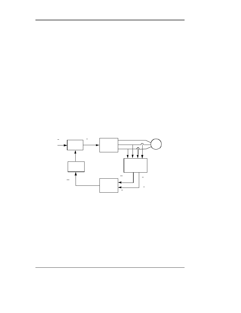
Field Orientation
41
Draft Date: February 5, 2002
Field orientation with respect to fluxes other than the rotor flux is also pos-
sible [23] with the stator and air gap fluxes being the most important alterna-
tives. Only the rotor flux yields complete decoupling, however, for some
purposes (wide range field weakening operation for example) the advantages
of choosing stator flux orientation can outweigh the lack of complete decou-
pling [24].
15.5.4
Direct Field Orientation
In direct field orientation the position of the flux to which orientation is desired
is directly measured using sensing coils or estimated from terminal measure-
ments. Since it is not possible to directly sense the rotor flux, a rotor flux-ori-
ented system must employ some type of computation to obtain the desired
information from a directly sensed signal. Figure 15.22 illustrates the nature of
these computations for terminal voltage and current sensing; the most fre-
quently used technique for direct field orientation.
In cases where flux amplitude information is available, a flux regulator can
be employed to improve the flux response. A variety of flux observers can be
employed to obtain improved response and less sensitivity to machine parame-
ters. Some of these are discussed in a later section. A major problem with most
direct orientation schemes is their inherent problems at very low speeds where
Figure 15.22 Direct field orientation with rotor field angle
θ
f
determined
from terminal voltage and current, “^” denotes estimate of a
motor parameter, “*” a commanded quantity,
σ
= 1 – L
m
2
/(L
r
L
s
)
i q d s
e
∗
i qds
s
cos
θ
f
sin
θ
f
λ
qds
e
i qds
s
v
qds
s
λ
q d s
s
v
q s
rˆ
1
–
i
qds
s
dt
∫
=
λ
q d r
s
L
ˆ
r
Lˆ
m
------
λ
ˆ
q d s
s
σ
ˆ Lˆ
s
i
q d s
s
–
[
]
=
Low-pass Filter
and
Transform
Open Loop
Rotor Flux
Observer
Flux Angle
Calculator
Coordinate
Transform
Current
Regulated
Amplifier
Induction
Motor
Torque
and Flux
Commands
Coordinate
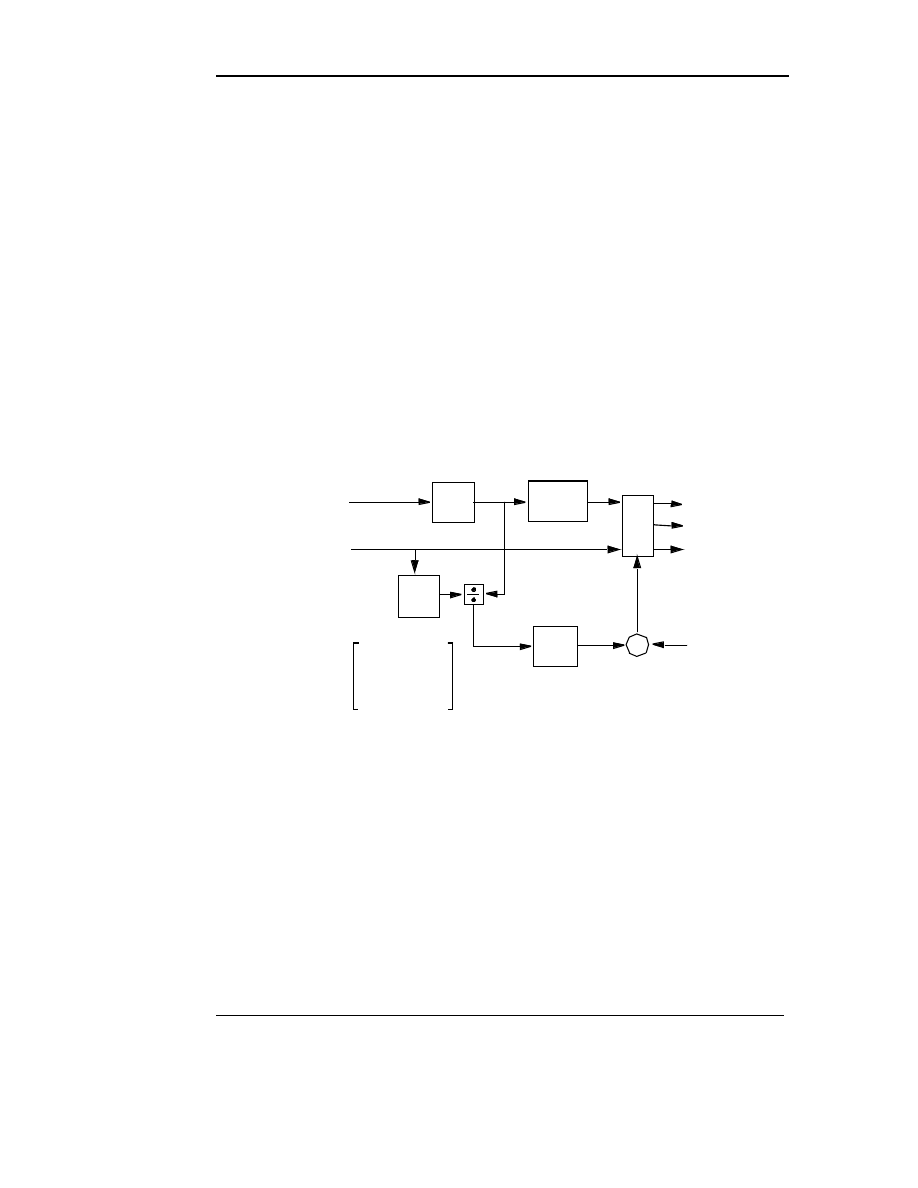
42
AC Motor Speed Control
Draft Date: February 5, 2002
the machine Ir drops are dominant and/or the required integration of signals
becomes problematic.
15.5.5
Indirect (Feedforward) Field Orientation
An alternative to direct sensing of flux position is to employ the slip relation,
Eq. (15.74), to estimate the flux position relative to the rotor. Figure 15.23
illustrates this concept and shows how the rotor flux position can be obtained
by adding the integral of the slip frequency calculated from the flux and torque
commands to the sensed rotor position to produce an angular estimate of the
rotor flux position. In the steady-state this approach corresponds to setting the
slip to the specific value which correctly divides the input stator current into
the desired magnetizing (flux producing) and secondary (torque producing)
currents. Indirect field orientation does not have inherent low-speed problems
and is thus preferred in most systems that must operate near zero speed.
15.5.6
Influence of Parameter Errors
Since knowledge of the machine parameters are a part of the feedback or feed-
forward controllers, both basic types of field orientation have some sensitivity
to machine parameters and provide non-ideal torque control characteristics
when control parameters differ from the actual machine parameters. In general
both steady-state torque control and dynamic response differ from the ideal
instantaneous torque control achieved by a correctly tuned controller.
Figure 15.23
Indirect field orientation controller using rotor flux and torque
producing current commands
i
as
*
i
bs
*
i
cs
*
λ
dr
e *
i
qs
e*
1
Tˆ
r
----
N
D
S
ω
e
*
i
ds
e*
1
L
ˆ
m
-----
1+pT
r
T
-1
θ
slip
θ
r
θ
f
*
1
p
--
T
1
–
θ
f
∗
cos
θ
f
∗
sin
θ
f
∗
sin
–
θ
f
∗
cos
=

Field Orientation
43
Draft Date: February 5, 2002
The major problem in the use of indirect control is the required knowledge
of the rotor open circuit time constant T
r
, which is sensitive to both temperature
and flux level [25]. When this parameter is incorrect in the controller the calcu-
lated slip frequency is incorrect and the flux angle is no longer appropriate for
field orientation. This results in an instantaneous error in both flux and torque
which can be shown to excite a second order transient characterized by eigen-
values having a real part equal to –1/T
r
and an oscillation frequency related to
the (incorrect) commanded slip frequency. Since T
r
is an open circuit time con-
stant and therefore rather large, these oscillations can be poorly damped. There
is also a steady-state torque amplitude error since the steady-state slip is also
incorrect. Steady state slip errors also cause additional motor heating and
reduced efficiency.
Direct field orientation systems are generally sensitive to stator resistance
and total leakage inductance, but the various systems have individual detuning
properties. Typically, parameter sensitivity is less than in indirect control, espe-
cially when a flux regulator is employed. In all cases, both direct and indirect,
parameter sensitivity depends on the ratio
σ
L
s
/r
1
with larger values giving
greater sensitivity. In the steady-state the quantity determines the location of
the peak torque and thus the shape of the torque versus slip frequency charac-
teristic. Thus, large, high efficiency machines tend to have high sensitivity to
parameter errors, and field weakened operation further aggravates this sensitiv-
ity.
15.5.7
Current Regulation
It has gradually been recognized that field oriented control allows speed loop
bandwidths far exceeding that of the DC motor (100 Hz or more) making
induction motor servos the device favored for demanding applications. How-
ever such a bandwidth can only be achieved with careful tuning of the current
regulator which serves to overcome the stator transient time constant. Current
regulators remain a rich area of research. However, the present methods can be
categorized generally as follows:
•
Sine-Triangle Current Regulation
•
Hysteresis Current Regulation
•
Predictive (dead-beat) Current Regulation.
The three types of regulators are illustrated in Figure 15.24.
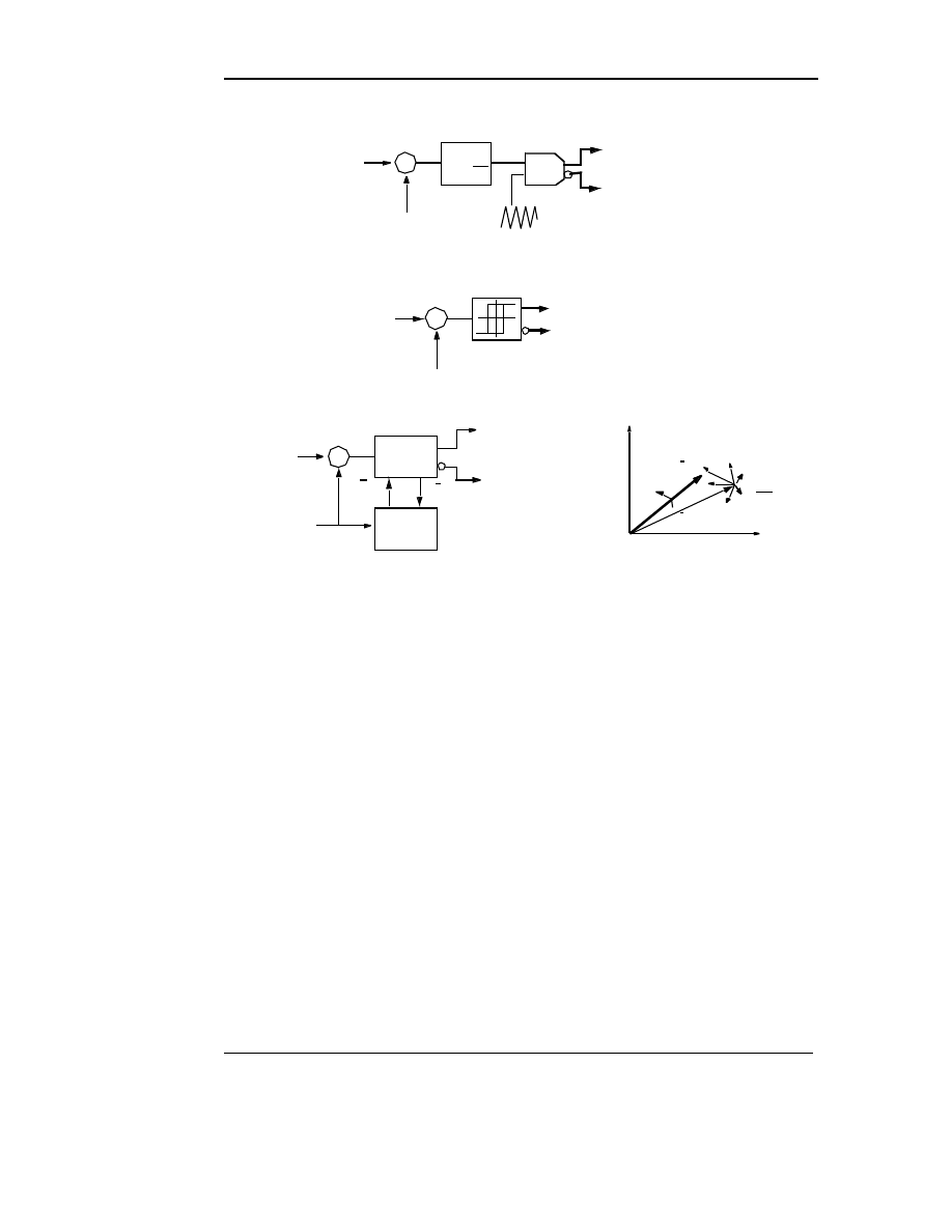
44
AC Motor Speed Control
Draft Date: February 5, 2002
The sine triangle intersection method uses the same basic principles as
sine-triangle pulse width modulation except that the input command to the
comparator is the error between a desired current value and the actual instanta-
neous value. Hence, the controller attempts to control the input current error to
zero. The current error in Figure 15.24(a) can be interpreted as the equivalent
to an instantaneous voltage command of zero in Figure 15.14. An advan-
tage of this controller is that the switching frequency is set by the triangle wave
frequency so that the harmonic structure is not appreciable altered when com-
pared with voltage PWM. Care must be taken however not to introduce exces-
sive proportional gain or added intersections command and triangle wave
could occur as a result of the harmonics introduced by the current feedback.
Excessive integrator gain on the other hand can cause oscillatory behavior.
Because of the phase shift introduced by the integrator, the current error of this
regulator can not be reduced to zero if the input command is sinusoidal (as is
Figure 15.24
Basic current regulation schemes, (a) three phase sine–
triangle comparison (b) three phase hysteresis control (c)
predictive regulation
Kp+Ki
s
Upper Switch
Lower Switch Logic
+
–
Triangle Wave
Comparator
Logic
(a)
+
–
Upper Switch
Lower Switch Logic
Logic
(b)
ia*
+
–
ia
Predictor
Model
ib ic
ib ic
* *
,
,
,
,
di
s
/dt
v
s
Lower Switch Logic
Upper Switch Logic
di
k
dt
∆
T
k=0,...6
is
is*
(c)
ia* ib ic
* *
,
,
ia* ib ic
* *
,
,
ia ib ic
,
,
ia ib ic
,
,
V
1
∗

Field Orientation
45
Draft Date: February 5, 2002
usually the case). Hence, the regulation is usually accomplished in the syn-
chronous frame, operating on current commands which becomes constant in
the steady state (see Section 15.5.2) [26].
The hysteresis regulator of Figure 15.24(b) produces switching whenever
the sign of the current error plus the hysteresis band changes polarity. The
proper setting of the hysteresis band is critical for this type of controller since
the band essentially sets the switching frequency. However, the frequency of
switching is not constant because the voltage producing a current change is
equal to the difference between the applied inverter voltage and the internal
EMF of the machine. Since the EMF varies sinusoidally throughout a cycle,
the pulse (switching) frequency varies throughout the cycle. Since the switch-
ing frequency becomes a variable dependant upon the instantaneous value of
back–EMF, the spectrum produced by the switching events are spread over a
continuous band of frequency and becomes difficult to predict. Thus, computa-
tion of motor losses produced by this type of input becomes very difficult.
Means for reducing the switching frequency variation have been reported [28],
[29] and work is ongoing.
The third type of current regulator is the predictive regulator of Figure
15.24(c). It can be recalled from Section 15.4.4 that switching of a three phase
inverter is characterized by only 8 state including two with zero voltage output.
Hence, only 7 unique switching states exist as shown in Figure 15.17. If the
future trajectory of the current is calculated just before each switching event
for all seven unique switch states, then the trajectory which directs the current
space vector in the best direction for tracking the commanded current can be
determined or predicted. Clearly the accuracy of the method is critically depen-
dant upon the motor model which is used to predict the current trajectory.
Many variations on this theme exist with Refs. [29] and [30] being a good
starting point.
15.5.8
“Sensorless” Speed Control
As AC motor drives have gradually matured, the cost and unreliability of
the speed/position encoder required for field oriented control has gradually
been recognized. Beginning with Joetten and Maeder [31], work has continued
on a myriad of alternatives to eliminate the speed/position sensor, many of
which have appeared in manufacturer’s equipment. In reality, of course, these
“sensorless” methods refer only to the fact that speed is not explicitly mea-

46
AC Motor Speed Control
Draft Date: February 5, 2002
sured but, rather, is inferred from electrical measurements and the machine
model.
As an introduction to the approach, the d–axis components of the squirrel
cage induction machine in a fixed, non-rotating frame “s” can be written, from
Section 15.5.2,
(15.78)
(15.79)
(15.80)
(15.81)
where and . Solving Eq. (15.81) for and sub-
stituting the result into Eq. (15.80),
(15.82)
where , or
(15.83)
The back emf of the d–axis rotor circuit is therefore
(15.84)
or, from Eq. (15.78)
(15.85)
In the same manner, for the q–axis emf
(15.86)
(15.87)
v
ds
s
r
1
i
d s
d
λ
d s
s
dt
-----------
+
=
0
r
2
i
d r
s
ω
r
λ
q r
s
d
λ
d r
s
dt
-----------
+
+
=
λ
d s
s
L
s
i
d s
s
L
m
i
dr
s
+
=
λ
d r
s
L
r
i
d r
s
L
m
i
ds
s
+
=
L
s
L
1
L
m
+
=
L
r
L
2
L
m
+
=
i
d r
s
λ
d s
s
L
m
L
r
------
λ
d r
s
σ
L
s
i
d s
s
+
=
σ
1
L
m
2
L
s
L
r
(
)
⁄
–
=
λ
d r
s
L
r
L
m
------
λ
d s
s
σ
L
r
L
s
L
m
-------------- i
ds
s
–
=
e
dr
s
d
λ
d r
s
dt
-----------
L
r
L
m
------
d
λ
d s
s
dt
-----------
σ
L
s
L
r
L
m
----------
di
d s
s
dt
---------
–
=
=
e
dr
s
L
r
L
m
------ v
d s
s
r
1
i
d s
s
–
(
) σ
L
s
L
r
L
m
----------
di
ds
s
dt
---------
–
=
λ
q r
s
L
r
L
m
------
λ
q s
s
σ
L
r
L
s
L
m
-------------- i
qs
s
–
=
e
qr
s
L
r
L
m
------ v
q s
s
r
1
i
q s
s
–
(
) σ
L
s
L
r
L
m
----------
di
qs
s
dt
---------
–
=
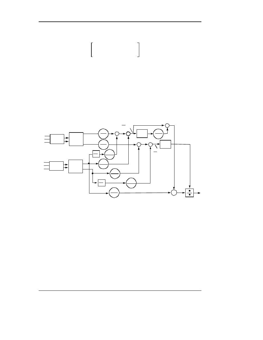
Induction Motor Observer
47
Draft Date: February 5, 2002
Finally, from Eq. (15.79), the rotor speed can now be expressed as
(15.88)
where, is obtained from Eq. (15.86), and from Eq. (15.85). A block
diagram of the complete speed sensor, developed previously in [32], is shown
in Figure 15.25. Clearly, perfect knowledge of all of the machine parameters
are needed to implement the approach which is rarely the case. However a rea-
sonable estimate of the parameters provide a speed estimate which is adequate
for moderate response speed control which does not include lengthy operation
near zero speed. A multitude of variations of this principle have appeared in
the literature which is nicely summarized in Ref. [32].
15.6 Induction Motor Observer
After 50 years of AC drive development the design of a sensorless induction
motor drive is still an engineering challenge. The basic problem is the need for
speed estimation which becomes especially difficult at low speed and under a
light load condition. The majority of speed identification methods rely on an
ω
r
1
λ
q r
s
------- r
2
λ
dr
s
L
r
-------
L
m
L
r
------i
d s
s
–
e
d r
s
–
=
λ
q r
s
e
dr
s
Figure 15.25 “Sensorless” sensing of rotor speed; mechanical speed in
rad./sec.
ω
rm
=
ω
r
/(P/2) where P is the number of poles
a, b, c
d–q
a, b, c
d–q
Filter
Filter
L
r
L
m
d
dt
r
2
L
m
L
r
r
2
L
r
v
as
v
bs
v
cs
i
a
i
b
i
c
d
dt
λ
dr
λ
dr
d
dt
λ
qr
λ
qr
L
r
L
m
v
ds
v
qs
to
to
d
dt
r
1
L
r
L
m
r
1
L
r
L
m
σ
L
s
L
r
L
m
σ
L
s
L
r
L
m
+
–
+
–
+
–
–
+
+
–
( )
∫
( )
∫
+
–
i
qs
i
ds
dt
dt
ω
ˆ
r

48
AC Motor Speed Control
Draft Date: February 5, 2002
approximate fundamental component model of the machine. The use of the sta-
tor equation, particularly the integration of the stator voltage vector, is com-
mon for all methods. Its solution is fairly accurate when the switched stator
voltage waveform is measured at high bandwidth and when the parameters that
determine the contributions of the resistive and the leakage voltage compo-
nents are well known. As the influence of these parameters dominates the esti-
mation at low speed, the steady state accuracy of speed sensorless operation
tends to be poor in during low or zero speeds.
One promising approach to solving this barrier is the sliding mode
approach to rotor flux and speed estimation of an induction machine. The slid-
ing mode method is a non-linear method for feedback control, state estimation
and parameter identification [33]. The property of the sliding mode approach is
due to use of straightforward fixed non-linear feedback control functions that
operate effectively over a specified magnitude range of system parameter vari-
ations and disturbances.
From Eq. (15.84) and (15.85) one can note that the rotor flux is related to
the stator voltage by
(15.89)
where the second two terms (Ir and leakage Ldi/dt drop) can be considered as
corrections to the major term, the applied d–axis voltage. This equation defines
what is called the voltage model. A similar equation applies for the q–axis cir-
cuit.
Alternatively the d–axis rotor flux can be calculated by combining Eqs.
(15.79) and (15.82) whereupon
(15.90)
In this case the input to the equation is the stator current and thus forms the
current model. Similar expressions for the q–axis rotor flux components can be
readily obtained.
In the interests of compactness it is convenient to cast these equations in
complex form, similar to Eqs. (15.54) and (15.55), as
L
m
L
r
------
d
λ
d r
s
dt
-----------
v
d s
s
i
d s
s
r
1
–
σ
L
s
di
d s
dt
---------
–
=
d
λ
dr
s
dt
-----------
ω
–
r
λ
qr
s
r
2
L
r
-----
λ
d r
s
–
r
2
L
m
L
r
------ i
d s
s
+
=

Induction Motor Observer
49
Draft Date: February 5, 2002
(voltage model)(15.91)
and
(current model) (15.92)
The most significant limitation of the rotor flux observer based on voltage
model is that it does not function at zero speed. At zero speed and low speed
the amplitude of the electromotive force is to small to accurately and reliably
determine the rotor flux angle necessary for both field orientation and speed
estimation. At low speed the flux estimation given by voltage model deterio-
rates owing to the effect of an inaccurate value of the stator resistance r
1
,
which causes a slight deviation of the rotor flux space vector. The current
model requires information about speed, so in a speed sensorless control one
needs to estimate both the rotor flux and mechanical speed.
To achieve an current based observer suitable for a sensorless drive, the the
observer control input should be a known function of motor speed so that, after
establishing a sliding mode in a torque tracking loop, the speed can be deter-
mined as unique solution [34]. Combining the voltage and current model,
(15.93)
where, the emf
(15.94)
A current estimation error can be defined as
(15.95)
and the carat “^” again denotes an estimate.
If the derivative in (15.95) is written in discretized form,
(15.96)
L
m
L
r
------
d
λ
q d r
s
dt
-------------
v
qds
s
i
qds
s
r
1
–
σ
L
s
di
qds
s
dt
-------------
–
=
d
λ
qdr
s
dt
-------------
j
ω
r
r
2
L
r
-----
–
λ
q d r
s
r
2
L
m
L
r
------ i
q d s
s
+
=
di
qds
s
dt
-------------
1
σ
L
s
--------- v
qds
s
r
1
i
q d s
s
–
L
m
L
r
------ e
qdr
s
r
2
L
m
L
r
------i
qds
s
+
–
=
e
qdr
s
j
ω
r
r
2
L
r
-----
–
λ
q d r
s
=
d
ε
i
dt
-------
d i
qds
s
iˆ
qds
s
–
(
)
dt
---------------------------------
1
σ
ˆ Lˆ
s
---------
L
m
L
r
------ e
q d r
s
eˆ
q d r
s
–
(
)
rˆ
1
rˆ
r
Lˆ
m
Lˆ
r
------
2
+
ε
i
⋅
–
=
=
d
ε
i
dt
-------
1
T
---
ε
i
k
( ) ε
i
k
1
–
(
)
–
[
]
=

50
AC Motor Speed Control
Draft Date: February 5, 2002
Equation (15.95) can be rewritten as
(15.97)
which can be rearranged to the form
(15.98)
Upon examining Eq. (15.98) it is clear that if the current error is driven
to zero then the error in the estimate of the emf is driven to zero. This observa-
tion can be employed to implement a controller which, by utilization of a cur-
rent regulated PWM algorithm (Figure 15.24) the current error can be driven to
zero. Hence, an estimate of the rotor back emf can be obtained.
A new updated value of emf at time step k based on the previous value at
time step k–1 plus the current estimation error can now be expressed as
(15.99)
where T is the length of the time step (sampling time) and
. The process of zeroing the error utilizing
current regulated PWM is the essence of sliding mode control.
A rotor flux observer can now be selected by utilizing Eq. (15.94), where-
upon, solving for the flux linkage
(15.100)
The speed estimate needed in Eq. (15.100) can be obtained from Figure 15.25.
A block diagram of the rotor flux algorithm is given in Figure 15.26. By
manipulation of the d–q machine equations other expressions for rotor linkage
and rotor speed are possible. For example one could use a simple integration of
Eq. (15.91), the voltage model, which performs well for speeds sufficiently far
from zero or (15.92), the current model, which is frequently used for low
ε
i
k
( ) ε
i
k
1
–
(
)
–
T
σ
ˆ Lˆ
s
---------
L
ˆ
m
L
ˆ
r
------ e
qdr
s
k
( )
eˆ
qdr
s
k
( )
–
[
]
rˆ
1
rˆ
2
Lˆ
m
Lˆ
r
------
2
+
ε
i
⋅
–
=
e
qdr
s
k
( )
eˆ
qdr
s
k
( )
–
σ
ˆ Lˆ
s
T
---------
Lˆ
m
Lˆ
r
------
1
T
σ
ˆ Lˆ
s
--------- rˆ
1
rˆ
2
Lˆ
m
Lˆ
r
------
2
+
+
ε
i
k
( ) ε
i
k
1
–
(
)
–
=
ε
i
k
( )
eˆ
qdr
k
( )
e
qdr
k
1
–
(
) σ
ˆ Lˆ
s
T
---------
Lˆ
r
Lˆ
m
------
1
TD
i
+
(
)ε
i
k
( ) ε
i
k
1
–
(
)
–
[
]
+
=
D
i
r
1
r
2
L
m
L
r
⁄
(
)
2
+
(
) σ
L
s
(
)
⁄
=
λ
q d r
s
j
ω
r
r
2
L
r
-----
+
ω
r
2
r
2
L
r
-----
2
+
--------------------------
–
e
qdr
s
=
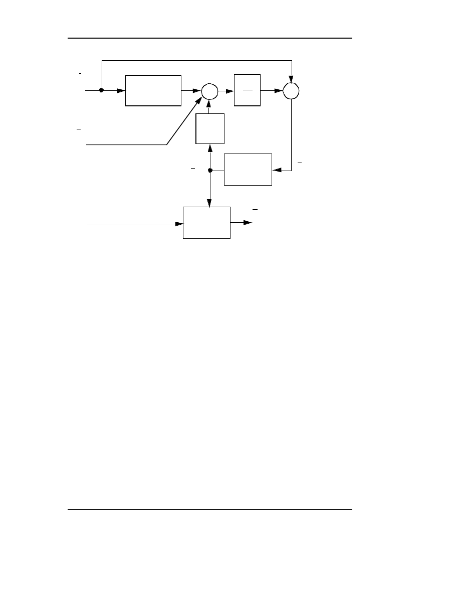
Permanent Magnet AC Machine Control
51
Draft Date: February 5, 2002
speeds. The reader is referred to the literature [32]–[34] for further informa-
tion.
15.7 Permanent Magnet AC Machine Control
15.7.1
Machine Characteristics
In contrast to induction machines which are overwhelmingly of the squirrel
cage construction, permanent magnet AC (PMAC) machines have been real-
ized in a variety of practical implementations depending upon stator winding
pattern, magnet disposition, air gap flux direction (radial, axial or a combina-
tion – transverse flux) and presence or absence of a rotor cage. However, two
broad categories can be identified 1) trapezoidal EMF machines and 2) sinuso-
idal EMF machines. The trapezoidal EMF machine is equipped with windings
concentrated into only one or at most a few full pitch slots per pole. The mag-
net disposition of these machines are usually located on the rotor surface and
generate a trapezoidal or rectangular EMF in the stator phase windings. The
span of the magnets are chosen so as to produce a quasi-rectangular
Figure 15.26 Closed loop rotor flux observer
rˆ
1
Lˆ
m
L
ˆ
r
------
2
rˆ
2
+
1
s
Eq. (15.99)
Lˆ
m
Lˆ
r
------
Eq.
(15.100)
i
qds
s
v
qds
s
–
–
+
+
+
λ
qdr
s
e
qdr
s
ε
i
ω
ˆ
r
Figure 15.25)
(from
120
°
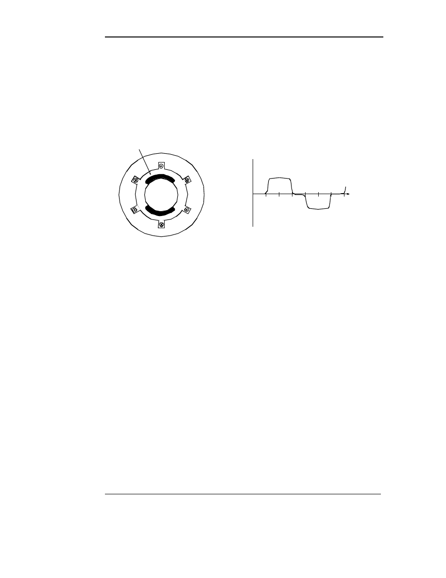
52
AC Motor Speed Control
Draft Date: February 5, 2002
waveform as shown in Figure 15.27. Since the EMF is rectangular, the optimal
stator current waveform is also quasi-rectangular. Rectangular currents are eas-
ily obtained by using only a single DC link current sensor and a relatively
crude position sensor which requires only a 6P pulses per revolution. However,
these machine are plagued with torque pulsation issues which are very compli-
cated due to the effects of armature reaction and are slowly being phased out in
favor of sinusoidal EMF machines.
While the stator windings of trapezoidal PMAC machines are concentrated
into narrow phase belts, the windings of a sinusoidal machine are typically dis-
tributed over multiple slots in order to approximate a sinusoidal distribution.
Whereas trapezoidal excitation strongly favors PMAC machines with non-
salient rotor designs (surface magnets) so that the phase inductances remain
constant as the rotor rotates so as to minimize the effects of armature reaction.
In contrast, PMAC machines with salient rotor poles can offer useful perfor-
mance characteristics when excited with sinusoidal EMF, providing flexibility
for adopting a variety of rotor geometries including a variety of inset or buried
magnet as alternatives to the baseline surface magnet design as shown in Fig-
ure 15.28.
The most convenient manner of analyzing a sinusoidal EMF PMAC
machine again uses instantaneous current, voltage, and flux linkage space vec-
tors in a reference frame fixed to the rotor flux presented in Section 15.5.2. In
this case the reference frame rotates synchronously with the applied stator field
so that the rotor speed in electrical radians per second . Referring to
Eqs. (15.57) to (15.62), these equations can be adapted to characterize a
Figure 15.27
Rectangular EMF PM machine utilizing surface magnets
+A
+B
+C
–C
–B
–A
EMF
ω
t
120ο
240ο
360ο
Magnet
ω
r
ω
e
=

Permanent Magnet AC Machine Control
53
Draft Date: February 5, 2002
PMAC machine by assuming that the flux produced by the d-axis rotor current
is constant. That is, an equivalent permanent magnet field is modeled when
,
(15.101)
Since no time varying currents flow in the rotor, the rotor equation, Eq.
(15.58), is not necessary when the rotor does not have a starting cage as is usu-
ally the case in a drive application. Combining Eqs. (15.57), (15.61) and
(15.101) and separating the complex stator equation into its two components
becomes, in scalar form, neglecting iron loss
(15.102)
(15.103)
In cases where the magnets are buried below the rotor surface as in Figure
15.28, the air gap inductances of the two axes must be modified to account for
the effect of saliency. With this modification, the equations for a buried magnet
machine in the steady state, wherein the p = d/dt terms are set to zero, become
(15.104)
(15.105)
Capital letters are used here to denote steady state conditions. As demonstrated
previously, the space vector equations and phasor equations are identical in the
steady-state except that space vector representation is usually interpreted in
terms of peak values whereas the phasor form is interpreted in terms of rms
quantities. A plot of the basic space vector (phasor) relation ships for the sinu-
Figure 15.28
Rotor configurations for four pole PMAC machines, (a)
inset, (b) interior radial flux and (c) interior circumferential
flux magnet orientation
(a)
(b)
(c)
L
m
i
d r
λ
m
constant
=
=
L
m
i
q r
0
=
v
qs
e
r
1
i
q s
e
p L
1
L
m
+
(
)
i
q s
e
ω
e
L
1
L
m
+
(
)
i
ds
e
ω
e
λ
m
+
+
+
=
v
ds
e
r
1
i
d s
e
p L
1
L
m
+
(
)
i
d s
e
ω
e
L
1
L
m
+
(
)
i
qs
e
–
+
=
V
q s
e
r
1
I
qs
e
ω
e
L
1
L
m d
+
(
)
I
d s
e
ω
e
Λ
m
+
+
=
V
d s
e
r
1
I
ds
e
ω
e
L
1
L
m q
+
(
)
I
q s
e
–
=
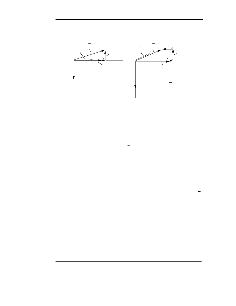
54
AC Motor Speed Control
Draft Date: February 5, 2002
soidal EMF PMAC machine is shown in Figure 15.29. The use of the super-
script “e” has been dropped for simplicity.
As indicated in Figure 15.29, the direct or d–axis has been aligned with the
permanent magnet flux linkage vector , so that the orthogonal quadrature or
q–axis is aligned with its time-rate-of change, the resulting back-EMF E
m
. The
amplitude of the back-EMF phasor E
m
can be expressed very simply as
(15.106)
where P is the number of pole pairs
ω
rm
is the mechanical speed in rad/s and
Λ
m
is the magnet flux linkage amplitude. The sinusoidal three-phase current
excitation is expressed in Figure 15.29 as an instantaneous current vector
made up of d– and q–axis scalar components i
d s
and i
qs
, respectively, and the
applied stator voltage phasor can be similarly depicted.
The value of magnetizing inductances L
md
will be smaller than L
mq
in
salient-pole PMAC machines using buried or inset magnets since the total
magnet thickness appears as an incremental air gap length in the d–axis mag-
netic circuit (i.e., for ceramic and rare earth magnet materials). Interior
PMAC machine designs of the type shown in Figure 15.28 with a single mag-
net barrier typically provide L
mq
/L
md
ratios in the vicinity of 3, while novel
laminated designs have been reported with saliency ratios of 7 or higher.
Figure 15.29
Basic steady-state relationships for sinusoidal PMAC
machine in synchronously rotating reference frame using d–
axis alignment with rotor magnet flux linkage , (a)
maximum torque per ampere, (b) unity power factor
Λ
m
−
j
Λ
m
E
m
=
ω
e
Λ
m
q-axis
d-axis
jx
q
I
q s
r
1
I
ds
I
qs
−
j
Λ
m
E
m
=
ω
e
Λ
m
q-axis
d-axis
jx
q
I
q s
r
1
I
s
I
s
V
s
V
s
(a)
(b)
V
s
= V
qs
–jV
ds
I
s
= I
qs
–jI
ds
jx
d
I
ds
x
q
=
ω
e
(L
1
+L
mq
)
x
d
=
ω
e
(L
1
+L
md
)
λ
m
E
m
ω
e
Λ
m
P
2
---
ω
r m
λ
m
=
=
I
s
V
s
µ
r
1
≅
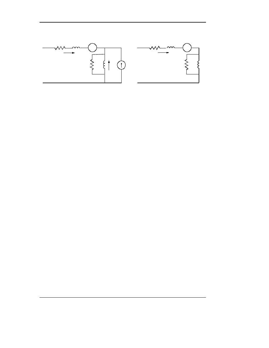
Permanent Magnet AC Machine Control
55
Draft Date: February 5, 2002
This d–q phasor representation leads to the following general expression
for the instantaneous torque developed in a sinusoidal PMAC machine,
(15.107)
where L
d
and L
q
are the d– and q–axis stator phase inductances, corresponding
to (L
md
+ L
1
) and (L
mq
+ L
1
), respectively, in the Figure 15.30 equivalent cir-
cuits. Since L
q
is typically larger than L
d
in salient pole PMAC machines, it is
worth noting that i
d s
and i
q s
must have opposite polarities for the second term
to contribute a positive torque component. The first “magnet” torque term is
independent of i
d s
but is directly proportional to stator current component i
q s
which is in phase with the back-EMF E
m
. In contrast, the second “reluctance”
torque term is proportional to the i
d s
.i
qs
current component product and to the
difference in the inductance values along the two axes (L
d
- L
q
). This interpre-
tation emphasizes the hybrid nature of the salient pole PMAC machine. Note
that the torque is no longer linearly proportional to the stator current amplitude
in the presence of magnetic circuit saliency.
15.7.2
Open-Loop V/Hz Control
As discussed briefly in Section 6.1.1, buried-magnet PMAC machines can be
designed with an induction motor squirrel cage winding embedded along the
surface of the rotor as sketched in Figure 15.31. This hybridization adds a com-
ponent of asynchronous torque production so that the PMAC machine can be
Figure 15.30
Coupled d–q equivalent circuits for a sinusoidal PMAC
machine in the synchronously rotating reference frame as
defined in Figure 6-22.
L
1
r
1
I
ds
V
ds
+
–
r
md
I
f
L
md
ω
e
λ
qs
+
−
L
1
r
1
I
q s
V
qs
+
–
r
mq
L
mq
ω
e
λ
ds
+
−
direct axis
quadrature axis
T
e
3
2
---
P
2
---
λ
m
i
q s
L
d
L
q
–
(
)
i
ds
i
q s
+
[
]
⋅
⋅
=

56
AC Motor Speed Control
Draft Date: February 5, 2002
operated stably from an inverter without position sensors. This simplification
makes it practical to use a simple constant volts-per-hertz (V/Hz) control algo-
rithm in much the same manner as for the induction machine. According to this
approach, a sinusoidal voltage PWM algorithm is implemented which linearly
increases the amplitude of the applied fundamental voltage amplitude in pro-
portion to the speed command to hold the stator magnetic flux approximately
constant. Compensation is again required for IR drop and for DC bus voltage
changes but, clearly, no compensation is needed for rotor slip.
The open loop nature of this control scheme makes it necessary to avoid
sudden large changes in the speed command or the applied load to avoid
undesired loss of synchronization (pull-out) of the PMAC machine. However,
an appealing aspect of this drive configuration is that the same constant volts-
per-hertz control approach can be used in many packaged induction motor
drives for general-purpose industrial speed control applications. Thus, cage-
type PMAC motors can be selected to replace induction motors in some adjust-
able speed drive applications to improve system operating efficiency without
changing the drive control electronics.
15.7.3
High-Performance Closed Loop Control.
In contrast to open loop operation, a rotor position sensor is typically required
to achieve high-performance motion control with the sinusoidal EMF PMAC
machine. The rotor position feedback needed to continuously perform the self-
synchronization function is essentially the same as an induction motor. How-
Figure 15.31
Cross section of a four pole PM/induction machine, showing
simplified block diagram of open loop volts per-hertz control
scheme.
Magnets
Squirrel Cage
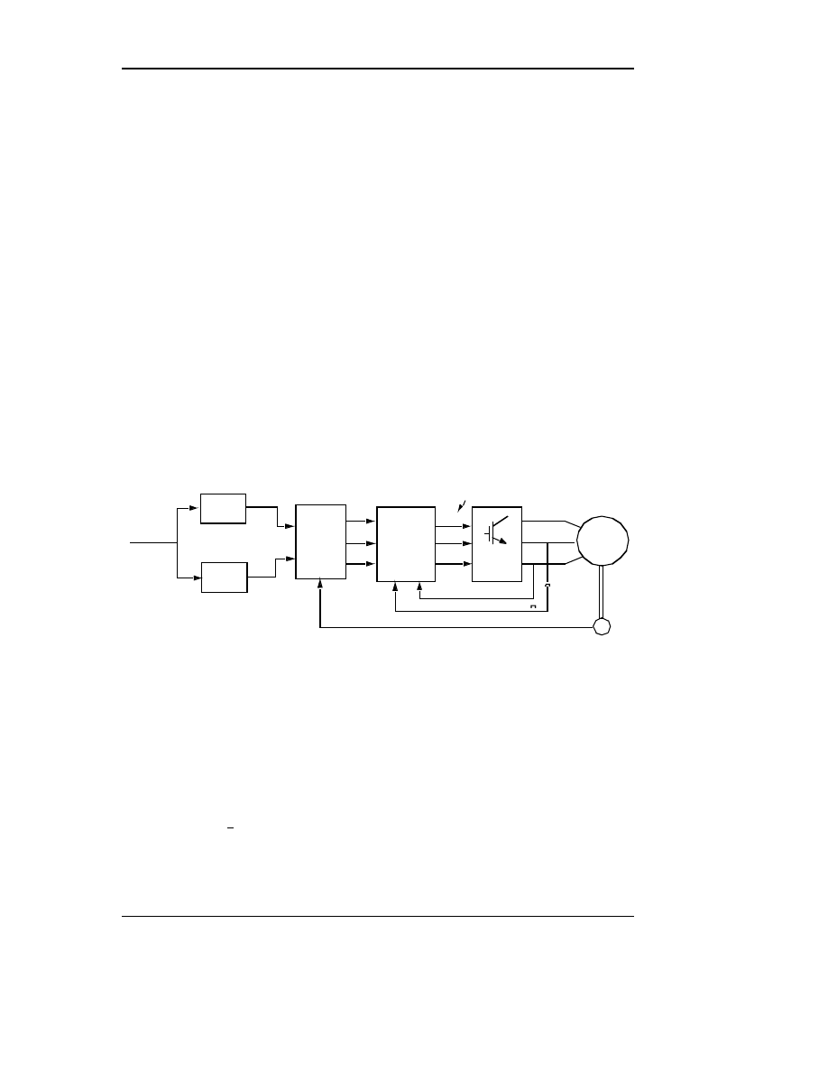
Permanent Magnet AC Machine Control
57
Draft Date: February 5, 2002
ever, cogging torque (torque pulsations) due to interaction of the magnets with
the stator slot harmonics places a heavier burden on the encoder to smooth out
these effects As result, an absolute encoder or resolver requiring a high resolu-
tion is frequently needed. In addition, in contrast to the induction machine, spe-
cial provision is frequently needed to provide smooth, controlled starting
performance since inappropriate energization at start can produce a brief nega-
tive rather than positive rotation.
One baseline approach for implementing this type of high-performance
torque control for sinusoidal PMAC machines is shown in Figure 6-25 [36].
According to this approach, the incoming torque command (asterisk des-
ignates command) is mapped into commands for d–q axis current components
and which are extracted from torque equation, Eq. (15.107). These
current commands in the rotor d–q reference frame (essentially DC quantities)
are then transformed into the instantaneous sinusoidal current commands for
the individual stator phases (i
a
*, i
b
*, and i
c
*) using the rotor angle feedback
θ
r
,
and the inverse vector rotation equations included as part of Figure 15.23.
The most common means of defining d–q current component commands
and as a function of the torque command into is to set a con-
straint of maximum torque-per-ampere operation which is nearly equivalent to
maximizing operating efficiency, see Figure 15.29. Trajectories of the stator
current vectors the rotor d–q reference frame which obey this maximum
torque-per-amp constraint are plotted in Figure 15.33 for a typical salient type
of PMAC machine. The trajectories are plotted over a range of torque ampli-
T
e
∗
i
d
∗
i
q
∗
Figure 15.32
Torque control scheme for sinusoidal PMAC motor
T
–1
(
θ
r)
PMAC
Motor
Current
Regulator
i
a
i
b
i
c
*
*
*
PWM
Inverter
d
a
d
b
d
c
Switching
Commands
Co-ordinate
Transformation
Te
*
f
d
(T
e
*)
f
q
(T
e
*)
i
ds
i
qs
*
*
θ
r
Position
Sensor
i
d s
∗
i
q s
∗
T
e
∗
i
qds
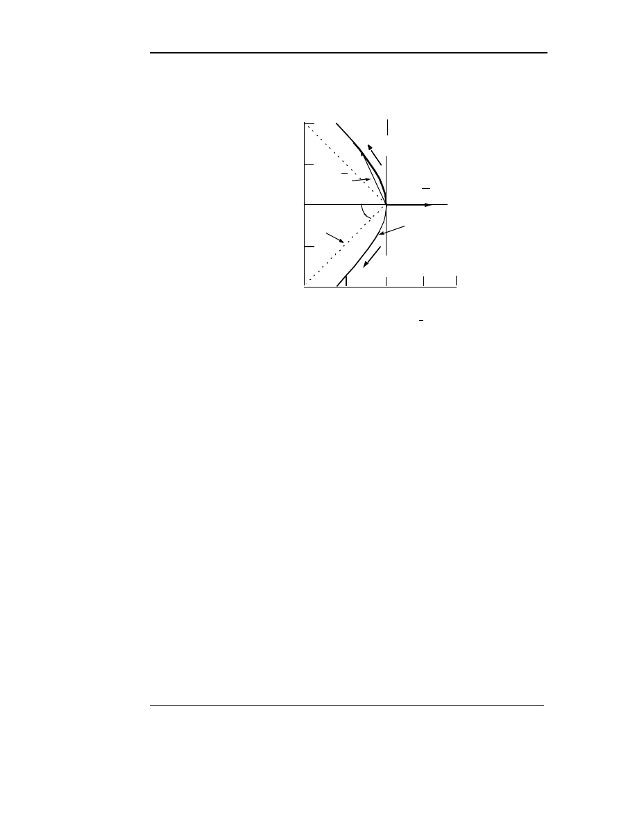
58
AC Motor Speed Control
Draft Date: February 5, 2002
tudes ranging from negative (generating/braking) to positive (motoring) values
[35].
It can be noted that the maximum torque-per-amp trajectory initially moves
along the q–axis for low values of torque before swinging symmetrically into
the second and third quadrant towards 45° asymptotes. For motoring operation,
this behavior means that maximum torque for a given amount of stator current
is developed by advancing the phase angle of the stator phase currents so that
they lead their respective back–EMF waveforms by angles between zero and
45° (electrical). The maximum torque-per-amp trajectory reflects the hybrid
nature of the PM machine having the capability of producing reluctance torque
as well as magnet torque. The corresponding currents I
d s
and I
q s
which define
the maximum torque per-amp trajectory for the salient pole PMAC machine
are plotted in Figure 15.34 [36].
Alternative field-oriented formulations of the sinusoidal PMAC machine
control algorithm have been reported that are also capable of achieving high
performance by aligning the rotating reference frame with the stator flux pha-
sor rather than with the rotor magnet flux [37],[38]. Although the performance
characteristics of these two control formulations are quite similar at low
speeds, their differences may become more apparent at higher speeds during
the transition from constant torque to constant horsepower operation.
Figure 15.33 Trajectory of stator current vector I
s
in the synchronous
reference frame as torque increases
+
T
e
Increasing
– T
e
Increasing
Typical I
s
Vector
I
d s
(Per Unit)
I
q
s
(
P
e
r
U
n
it
)
– 1.0
– 0.5
0
0.5
1.0
– 1.0
– 0.5
0
0.5 1.0
45
o
Locus of Current
Vector I
s
ψ
f
Asymptote
d-axis
q-axis
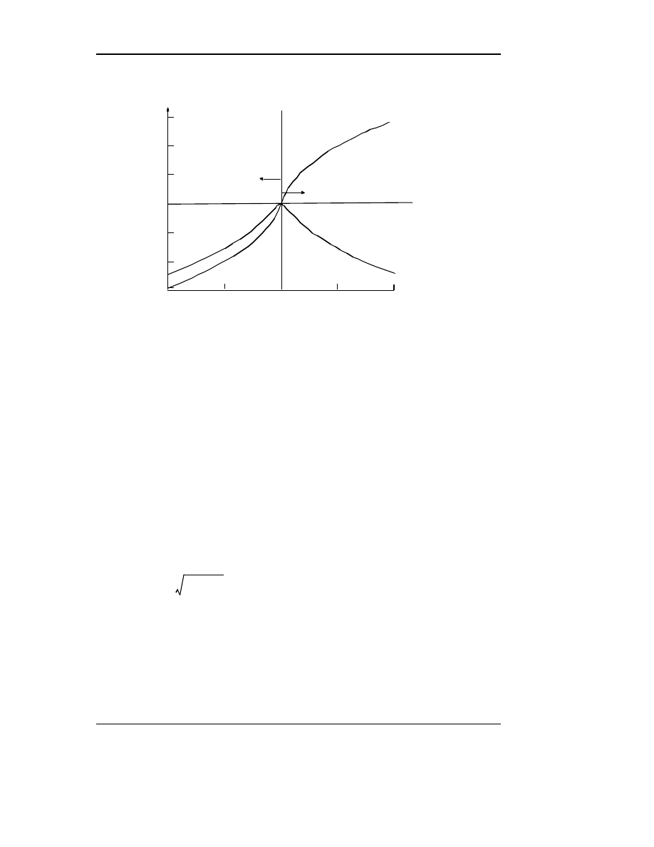
Permanent Magnet AC Machine Control
59
Draft Date: February 5, 2002
15.7.4
Regenerative Braking Operation.
Figure 15.34 shows that the maximum torque-per-amp trajectories are mirror
images in the second and third quadrants. Stated in a different way, the I
q s
function plotted in Figure 15.34 is sensitive to the polarity of the torque com-
mand, while the I
ds
function depends only on its absolute value.
15.7.5
Field Weakening
The load torque limits in the speed range from zero to rated speed is set by the
maximum current that can be supplied from the inverter, that is
(15.108)
The limiting value of Eq. (15.108) can be visualized as a circle in the i
ds
–i
q s
plane centered at the origin with radius I
max
.
Beyond rated speed another constraint is imposed since the inverter pulse
width modulator saturates and the output voltage becomes a constant. In this
case, clearly
Figure 15.34 Direct and quadrature axis stator currents required to
produce maximum torque per ampere for a salient pole
permanent magnet machine
Torque T
e
(Per Unit)
I
d
I
q
Id
s,
I
q
s
(P
e
r
U
n
it
)
Generating/Braking
Region
Motoring Region
– 10
– 5
0
5
10
– 3
– 2
– 1
0
1
2
3
I
q s
2
I
ds
2
+
I
max
≤

60
AC Motor Speed Control
Draft Date: February 5, 2002
(15.109)
Using Eqs. (15.104) and (15.105) and rearranging the result, (15.109) can be
expressed as
(15.110)
Eq. (15.110) can be visualized as a second ellipse in the i
ds
–i
qs
plane with a
focal point at i
qs
= 0 and i
d s
= -
λ
m
/L
d s
. The size of the ellipse continues to
decrease as the speed (
ω
r
=
ω
e
) increases.
Control of the d-q currents in the field weakening range must be such that
the current remains in the circle of Eq. (15.108) and tracks along the shrinking
elliptical boundary as shown in Figure 15.35. It can be noted that the d–axis
current is driven negative implying a stator MMF component acting to reduce
the magnet flux (demagnetize the magnet). When I
d s
becomes equal to
λ
m
/L
d s
,
the flux in the magnet has been driven to zero. Further negative increases in I
d s
must now be prevented. As a result the torque producing component I
qs
now
begins to decrease rapidly and constant horsepower operation can no longer be
maintained. The field weakening region in Figure 15.35 corresponds to the
segment from point A to point B.
References
[1]
F.M.H. Khater and D.W. Novotny, “An equivalent circuit model for
phase back voltage control of AC machines, IEEE Transactions on
Industry Applic., vol. 22, no. 5, Sept./Oct., pp. 835-841
[2]
T.A. Lipo, “The analysis of induction motors with voltage control by
symmetrically triggered thyristors”, IEEE Trans. on Power Apparatus
and Systems, vol. PAS-90, no. 2, March/April 1971, pp.515-525.
[3]
J. Davoine, R. Perret and H. Le-Huy, “Operation of a self-controlled syn-
chronous motor without a shaft position sensor”, in Conf. Rec. IEEE IAS
Annual Meeting, 1981, pp. 696-701.
[4]
J. Holtz and S. Stadtfeld, “A predictive controller for the stator current
vector of ac machines fed from a switched voltage source”, in Conf. Rec.
IPEC Conf, Tokyo, 1983, pp. 1665-1675.
V
qs
2
V
d s
2
+
V
max
≤
2
π
--- V
bus
=
2
π
---
V
b u s
ω
e
----------
i
qs
2
L
d s
L
q s
-------
2
i
ds
λ
m
L
d s
-------
+
2
+
=
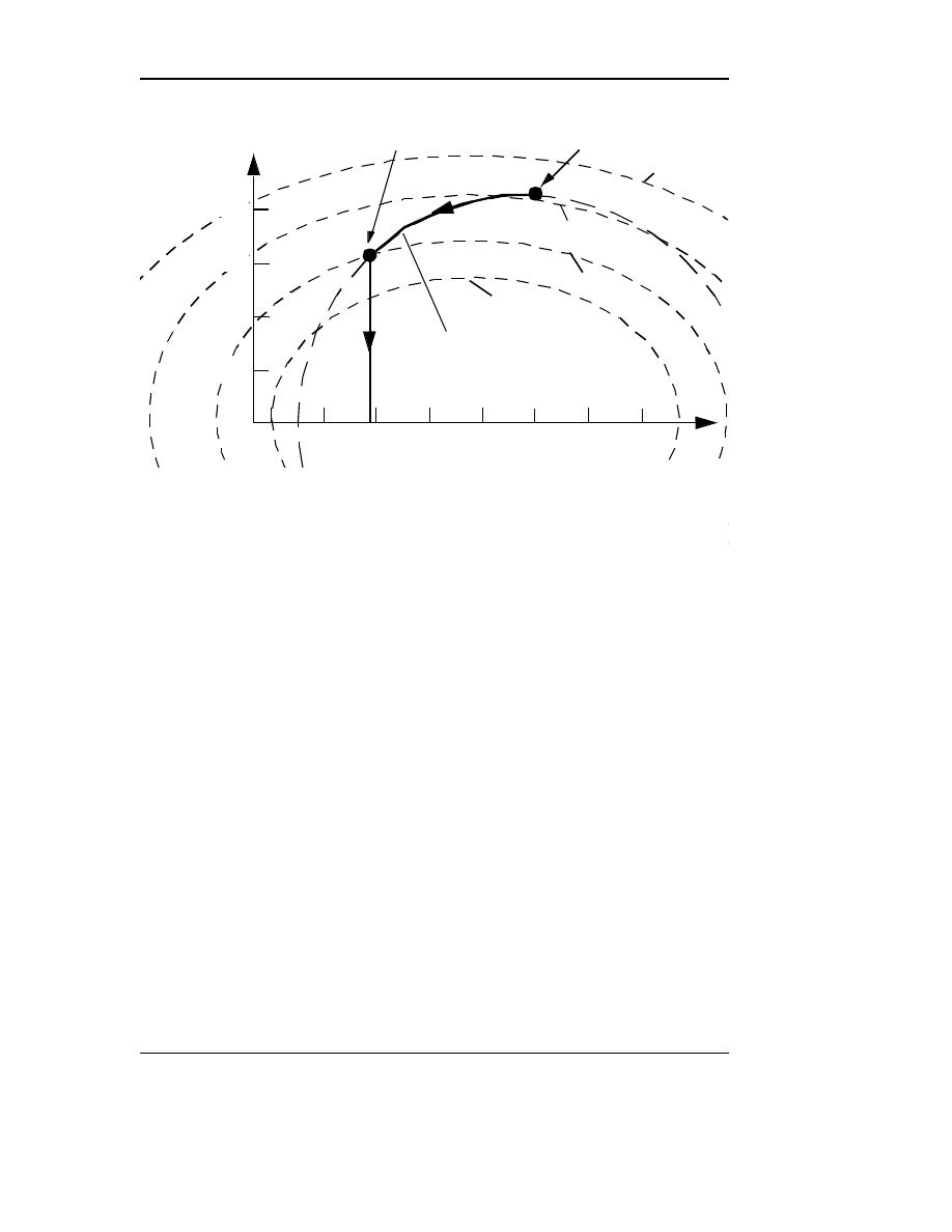
Permanent Magnet AC Machine Control
61
Draft Date: February 5, 2002
[5]
H.W. Van der Broeck, H. Skudelny and G. Stanke, “Analysis and realiza-
tion of a pulse width modulator based on voltage space vectors”, IEEE
Trans. on Industry Applications., vol. 24, no. 1, Jan./Feb., 1988, pp. 142-
150.
[6]
B. Mokrytzki, “The controlled slip static inverter drive”, IEEE Trans. On
Industry and General Applications, vol. IGA-4, May/June 1968, pp. 312-
317.
[7]
K. Koga, R. Ueda and T. Sonoda, “Achievement of high performances
for general purpose inverter drive induction motor system”, in Conf. Rec.
IEEE IAS Annual Meeting, 1989, pp. 415-425.
[8]
F. Blaabjerg and J.K. Pedersen, “Ideal PWM–-VSI inverter using only
one current sensor in the DC–link”, in Conf. Rec. IEE 5th Power Elec-
tronics and Variable–-Speed Drives Conf., 1994, pp. 458-464.
[9]
S.I. Moon and A. Keyhani, “Estimation of induction machine parameters
from standstill time-domain data”, IEEE Trans. on Industry Applic, vol.
30, no. 6, 1994, pp. 1609-1615
Figure 15.35 Locus of current vector in the d–q plane during operation
above rated speed (constant horsepower region is A–B)
I
qs
(P.U.)
I
ds
(P.U.)
0
λ
m
L
d s
-------
–
End of Const; Torque
End of Const. Horsepower Mode
ω
r
=
ω
1
ω
2
>
ω
1
ω
3
>
ω
2
ω
4
>
ω
3
Current Limit
0.5
0.5
–0.5
-1.0
1.0
0.75
0.25
A
B

62
AC Motor Speed Control
Draft Date: February 5, 2002
[10] J. Stephan, M. Bodson and J. Chaisson, “Real-time estimation of the
parameters and fluxes of induction motors”, IEEE Trans. on Industry
Applic., vol. 30, no. 3, 1994, pp. 746-758.
[11] J.A. Capolino, “Identification of induction machine parameters”, in Conf.
Rec. of the Int. Aegean Conf. on Electric Machines and Power Electron-
ics, vol. 2, 1995, pp. 627-637.
[12] Y. Kishimoto, S. Asaba, K. Nakata and S. Kawatsu, “Control device for
induction motor”, U.S. Patent 5,231,339, July 27, 1993.
[13] S.I Moon and A. Keyhani, “Estimation of induction machine parameters
from standstill time-domain data”, IEEE Trans. on Industry Applications,
vol. 30, no. 6, 1994, pp. 1609-1615.
[14] J. Stephan, M. Bodson and J. Chaisson, “Real-time estimation of the
parameters and fluxes of induction motors”, IEEE Trans. on Industry
Applications, vol. 30, no. 3, 1994, pp. 746-758.
[15] J.A. Capolino, “Identification of induction machine parameters”, Proc. of
the Int. Aegean Conf. on Electrical Machines and Power Electronics, vol.
2, 1995, pp. 627-637.
[16] A. Munoz-Garcia, T.A. Lipo and D.W. Novotny, “A new induction motor
open-loop speed control capable of low frequency operation”, IEEE
Trans. on Industry Applications, vol. 34, no. 5, July/August, pp. 813-821.
[17] D. Leggate and R. Kerkman, “Pulse based time compensator for PWM
voltage inverters”, in Conf. Record of IEEE IECON, 1995, pp. 474-481.
[18] J.W. Choi, S.I. Yong and S.K. Sul, “Inverter output voltage synthesis
using novel dead time compensation”, IEEE Trans. on Industrial Applic.,
vol. 31, no. 5, 1995, pp. 1001-1008.
[19] Y. Murai, T. Watanabe and H. Iwasaki, “Waveform distortion and correc-
tion circuit for PWM inverters with switching lag-times”, IEEE Trans. on
Industrial Applic., vol. 23, no. 5, 1987, pp. 881-886.
[20] T. Sukegawa, K. Kamiyama, T. Matsui, and T. Okuyama, “Fully digital,
vector controlled PWM-VSI fed AC drives with an inverter dead-time
compensation strategy”, in Conf. Rec. IEEE IAS Annual Mtg., 1988, pp.
463-469.

Permanent Magnet AC Machine Control
63
Draft Date: February 5, 2002
[21] J.W. Choi, S.I. Yong and S.K. Sul, “Inverter output voltage synthesis
using novel dead time compensation”, in Conf. Rec. IEEE IAS Annual
Mtg., 1994, pp. 100-106.
[22] D.W. Novotny and T.A. Lipo, “Vector control and dynamics of AC
drives”, (book) Oxford Press, Oxford England, 1996.
[23] R. de Doncker and D.W. Novotny, “The universal field oriented control-
ler”, in Conf. Rec. IEEE IAS Annual Meeting, Oct. 1988, p. 450-456.
[24] X. Xu and D.W. Novotny, “Selection of the flux reference for induction
machines in the field weakening region”, IEEE Trans. on Industry
Applic., vol. 28, no. 6, November/December 1992, pp. 1353-1358.
[25] K.B. Nordin, D.W. Novotny and D.S. Zinger, “The influence of motor
parameter deviations in feedforward field orientation drives systems”,
IEEE Trans. in Industry Applic., vol. IA-21, no. 4, July/August 1985, pp.
1009-1015.
[26] T. Rowan and R. Kerkman, “A new synchronous current regulator and an
analysis of current-regulated PWM inverters”, IEEE Trans. on Industry
Applic., vol. IA-22, no. 4, July/August 1986, pp. 163-171.
[27] L. Malesani and P. Tenti, “A novel hysteresis control method for current
controlled VSI PWM with constnat switching frequency”, IEEE Treans.
onm Industry Applic., vol. IA-26, no. 1, Jan/Feb, 1990, pp. 88-92.
[28] Q. Yao and D.G. Holmes, “A simple, novel method for variable-hystere-
sis-band current control of a three phase inverter with constant switching
frequency”, in Conf. Rec. IEEE IAS Annual Meeting, 1993, pp. 1122-
1129.
[29] J. Holtz and S. Stadtfeld, “A predictive controller for the stator current
vector of AC machines fed from a switched voltage source”, in Conf.
Rec. IPEC, Tokyo, 1983, pp. 1665-1675.
[30] A. Nabae, S. Ogasawara and H. Akagi, “A novel control scheme for cur-
rent-controlled PWM inverters”, IEEE Trans. on Industry Applic., vol.
22, no. 4, JulyAugust, 1986, pp. 697-701.
[31] R. Joetten and G. Maeder, “Control methods for good dynamic perfor-
mance induction motor drives based on current and voltage as measured
quantities”, IEEE Transactions on Industry Applic., vol. IA-19, no. 3,
May/June 1983, pp. 356-363.

64
AC Motor Speed Control
Draft Date: February 5, 2002
[32] K. Rajashekara, A. Kawamura and K. Matsuse (editors), “Sensorless
control of AC motor drives”, (book) IEEE Press, 1996.
[33] V.I. Utkin, “Sliding mode control design principles and applications to
electric drives”, IEEE Trans. on Ind. Elec., Vol.40, 1993, pp.23-36.
[34] M. Rodic, K. Jezernik, A. Sabanovic, “Speed sensorless sliding mode
torque control of induction motor”, in Conf. Rec. IEEE-IAS Ann. Meet-
ing, 2000, pp.1820-1827.
[35] S. Morimoto, Y. Takeda, T. Hirasa and K. Taniguchi, “Expansion of oper-
ating limits for PM motor by optimum flux weakening”, IEEE Trans. on
Industrial Applic., vol. 26, no. 5, Sept.Oct. 1990, pp. 866-871.
[36] T.M. Jahns, G.B. Kliman and T.W. Neumann, “Interior PM synchronous
motors for adjustable-speed drives”, IEEE Trans. on Industrial Applic.,
vol. 22, no. 4, July/August 1986, pp. 738-747.
[37] B.K. Bose, “A high-performance inverter-fed drive system of an interior
PM synchronous machine”, IEEE Trans. on Industrial Applic., vol. 24,
no. 6, Nov./Dec. 1988, pp. 987-998.
[38] M.A. Bilewski, A. Fratta, L. Giordano, A. Vagati and F. Villata, “Control
of high performance interior PM synchronous drives”, in Conf. Rec.
IEEE-IAS Annual Meeting, 1990, pp. 531-538.
Wyszukiwarka
Podobne podstrony:
hydroform control id 207652 Nieznany
4533 ac id 38899 Nieznany (2)
4115 ac id 38554 Nieznany (2)
870 ac id 47710 Nieznany (2)
controlling (9 stron) id 119256 Nieznany
IEEE PCA AC Motor Application 0 Nieznany
4506 ac id 514788 Nieznany (2)
Controlling bankowy 2 id 119273 Nieznany
4061 ac id 38409 Nieznany (2)
475 ac id 39057 Nieznany (2)
zywnosc wygodna AC id 107133 Nieznany
ControlLogix L7x id 119373 Nieznany
emcephob ac id 160689 Nieznany
4533 ac id 38899 Nieznany (2)
4115 ac id 38554 Nieznany (2)
Abolicja podatkowa id 50334 Nieznany (2)
4 LIDER MENEDZER id 37733 Nieznany (2)
więcej podobnych podstron