
MATLAB
R
°
/ R Reference
November 24, 2009
David Hiebeler
Dept. of Mathematics and Statistics
University of Maine
Orono, ME 04469-5752
http://www.math.umaine.edu/~hiebeler
I wrote the first version of this reference during the Spring 2007 semester, as I learned R while teaching
my course “MAT400, Modeling & Simulation” at the University of Maine. The course covers population
and epidemiological modeling, including deterministic and stochastic models in discrete and continuous
time, along with spatial models. Half of the class meetings are in a regular classroom, and half are in
a computer lab where students work through modeling & simulation exercises. When I taught earlier
versions of the course, it was based on Matlab only. In Spring 2007, some biology graduate students in
the class who had learned R in statistics courses asked if they could use R in my class as well, and I said
yes. My colleague Bill Halteman was a great help as I frantically learned R to stay ahead of the class.
As I went, every time I learned how to do something in R for the course, I added it to this reference, so
that I wouldn’t forget it later. Some items took a huge amount of time searching for a simple way to do
what I wanted, but at the end of the semester, I was pleasantly surprised that almost everything I do
in Matlab had an equivalent in R. I was also inspired to do this after seeing the “R for Octave Users”
reference written by Robin Hankin. I’ve continued to add to the document, with many additions based
on topics that came up while teaching courses on Advanced Linear Algebra and Numerical Analysis.
This reference is organized into general categories. There is also a Matlab index and an R index at
the end, which should make it easy to look up a command you know in one of the languages and learn
how to do it in the other (or if you’re trying to read code in whichever language is unfamiliar to you,
allow you to translate back to the one you are more familiar with). The index entries refer to the item
numbers in the first column of the reference document, rather than page numbers.
Any corrections, suggested improvements, or even just notification that the reference has been useful
will be appreciated. I hope all the time I spent on this will prove useful for others in addition to myself
and my students. Note that sometimes I don’t necessarily do things in what you may consider the “best”
way in a particular language; I often tried to do things in a similar way in both languages. But if you
believe you have a “better” way (either simpler, or more computationally efficient) to do something, feel
free to let me know.
Acknowledgements: Thanks to Alan Cobo-Lewis and Isaac Michaud for correcting some errors;
and Thomas Clerc, Richard Cotton, Stephen Eglen, Andreas Handel, David Khabie-Zeitoune, Michael
Kiparsky, Andy Moody, Lee Pang, Manas A. Pathak, Rune Schjellerup Philosof, and Corey Yanofsky for
contributions.
Permission is granted to make and distribute verbatim copies of this manual provided this permission
notice is preserved on all copies.
Permission is granted to copy and distribute modified versions of this manual under the conditions
for verbatim copying, provided that the entire resulting derived work is distributed under the terms of a
permission notice identical to this one.
Permission is granted to copy and distribute translations of this manual into another language, un-
der the above conditions for modified versions, except that this permission notice may be stated in a
translation approved by the Free Software Foundation.
Copyright c
°2007–2009 David Hiebeler
1

D. Hiebeler, Matlab / R Reference
2
Contents
1 Help
3
2 Entering/building/indexing matrices
3
2.1
Cell arrays and lists . . . . . . . . . . . . . . . . . . . . . . . . . . . . . . . . . . . . . . .
6
2.2
Structs and data frames . . . . . . . . . . . . . . . . . . . . . . . . . . . . . . . . . . . . .
6
3 Computations
6
3.1
Basic computations . . . . . . . . . . . . . . . . . . . . . . . . . . . . . . . . . . . . . . . .
6
3.2
Complex numbers . . . . . . . . . . . . . . . . . . . . . . . . . . . . . . . . . . . . . . . .
7
3.3
Matrix/vector computations . . . . . . . . . . . . . . . . . . . . . . . . . . . . . . . . . . .
8
3.4
Root-finding . . . . . . . . . . . . . . . . . . . . . . . . . . . . . . . . . . . . . . . . . . . .
14
3.5
Function optimization/minimization . . . . . . . . . . . . . . . . . . . . . . . . . . . . . .
14
3.6
Numerical integration / quadrature . . . . . . . . . . . . . . . . . . . . . . . . . . . . . . .
15
3.7
Curve fitting . . . . . . . . . . . . . . . . . . . . . . . . . . . . . . . . . . . . . . . . . . .
16
4 Conditionals, control structure, loops
17
5 Functions, ODEs
21
6 Probability and random values
23
7 Graphics
27
7.1
Various types of plotting . . . . . . . . . . . . . . . . . . . . . . . . . . . . . . . . . . . . .
27
7.2
Printing/saving graphics . . . . . . . . . . . . . . . . . . . . . . . . . . . . . . . . . . . . .
35
7.3
Animating cellular automata / lattice simulations . . . . . . . . . . . . . . . . . . . . . . .
36
8 Working with files
37
9 Miscellaneous
38
9.1
Variables . . . . . . . . . . . . . . . . . . . . . . . . . . . . . . . . . . . . . . . . . . . . .
38
9.2
Strings and Misc. . . . . . . . . . . . . . . . . . . . . . . . . . . . . . . . . . . . . . . . . .
39
10 Spatial Modeling
42
Index of MATLAB commands and concepts
43
Index of R commands and concepts
48

D. Hiebeler, Matlab / R Reference
3
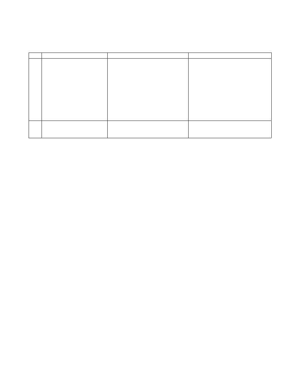
1
Help
No.
Description
Matlab
R
1
Show help for a function (e.g.
sqrt)
help sqrt
, or helpwin sqrt to see
it in a separate window
help(sqrt)
or ?sqrt
2
Show help for a built-in key-
word (e.g. for)
help for
help(’for’)
or ?’for’
3
General list of many help top-
ics
help
library()
to see available libraries,
or library(help=’base’) for very
long list of stuff in base package which
you can see help for
4
Explore main documentation
in browser
doc
or helpbrowser (previously it
was helpdesk, which is now being
phased out)
help.start()
5
Search
documentation
for
keyword or partial keyword
(e.g. functions which refer to
“binomial”)
lookfor binomial
help.search(’binomial’)
2
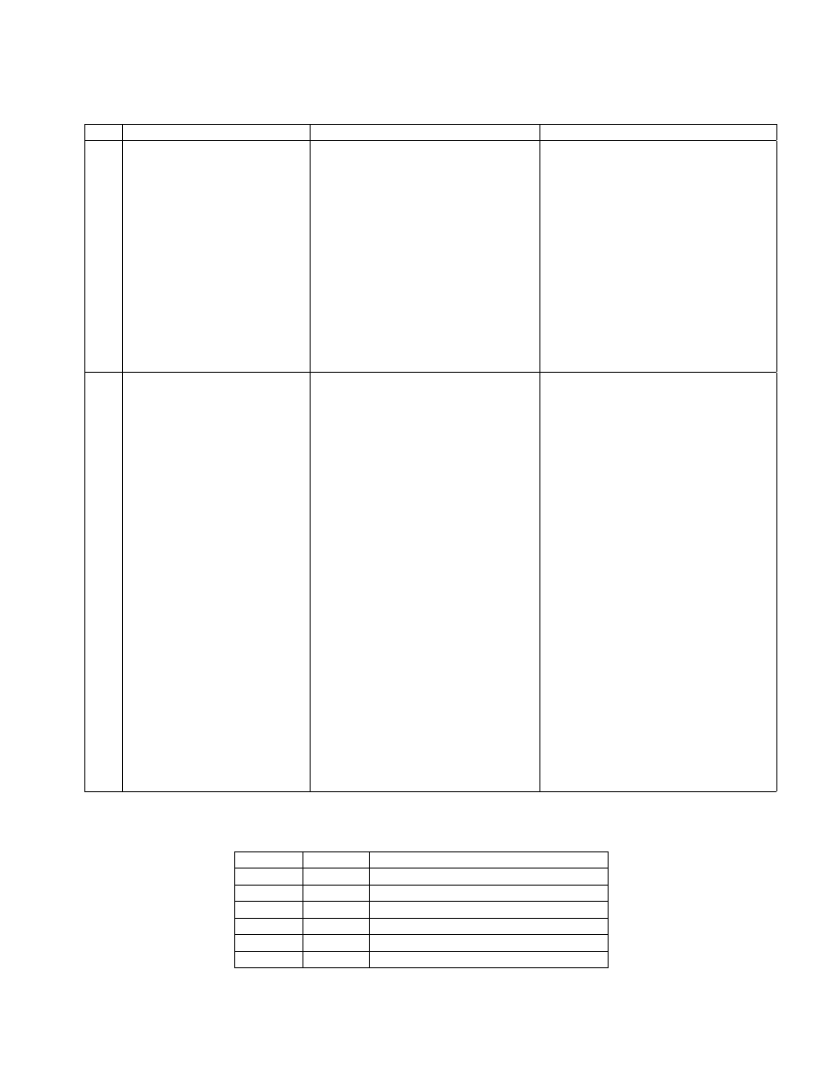
Entering/building/indexing matrices
No.
Description
Matlab
R
6
Enter a row vector ~v
=
£
1
2 3 4
¤
v=[1 2 3 4]
v=c(1,2,3,4)
or
alternatively
v=scan()
then enter “1 2 3 4” and
press Enter twice (the blank line
terminates input)
7
Enter a column vector
1
2
3
4
[1; 2; 3; 4]
c(1,2,3,4)
(R does not distinguish between row
and column vectors.)
8
Enter a matrix
·
1 2
3
4 5
6
¸
[1 2 3 ; 4 5 6]
To
enter
values
by
row:
matrix(c(1,2,3,4,5,6), nrow=2,
byrow=TRUE)
To enter values by
column:
matrix(c(1,4,2,5,3,6),
nrow=2)
9
Access an element of vector v
v(3)
v[3]
10
Access an element of matrix
A
A(2,3)
A[2,3]
11
Access an element of matrix
A using a single index: in-
dices count down the first col-
umn, then down the second
column, etc.
A(5)
A[5]
12
Build the vector [2 3 4 5 6 7]
2:7
2:7
13
Build the vector [7 6 5 4 3 2]
7:-1:2
7:2
14
Build the vector [2 5 8 11 14]
2:3:14
seq(2,14,3)

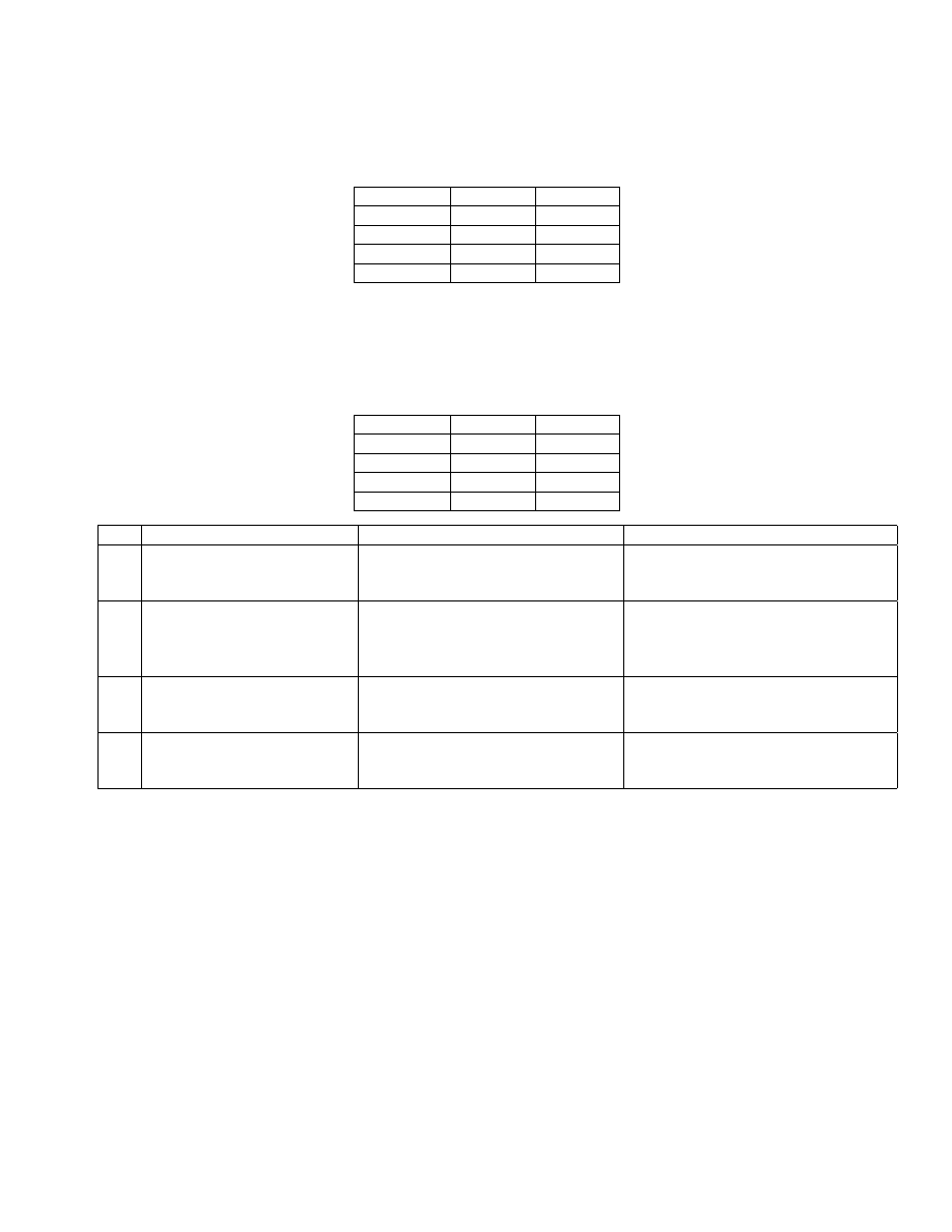
D. Hiebeler, Matlab / R Reference
4
No.
Description
Matlab
R
15
Build a vector containing
n equally-spaced values be-
tween a and b inclusive
linspace(a,b,n)
seq(a,b,length.out=n)
or
just
seq(a,b,len=n)
16
Build a vector containing
n
logarithmically
equally-
spaced values between 10
a
and 10
b
inclusive
logspace(a,b,n)
10^seq(a,b,len=n)
17
Build a vector of length k
containing all zeros
zeros(k,1)
(for a column vector) or
zeros(1,k)
(for a row vector)
rep(0,k)
18
Build a vector of length k
containing the value j in all
positions
j*ones(k,1)
(for a column vector)
or j*ones(1,k) (for a row vector)
rep(j,k)
19
Build an m×n matrix of zeros
zeros(m,n)
matrix(0,nrow=m,ncol=n)
or just
matrix(0,m,n)
20
Build an m × n matrix con-
taining j in all positions
j*ones(m,n)
matrix(j,nrow=m,ncol=n)
or just
matrix(j,m,n)
21
n × n identity matrix I
n
eye(n)
diag(n)
22
Build diagonal matrix A us-
ing elements of vector v as di-
agonal entries
diag(v)
diag(v,nrow=length(v))
(Note: if
you are sure the length of vector v is 2
or more, you can simply say diag(v).)
23
Extract diagonal elements of
matrix A
v=diag(A)
v=diag(A)
24
“Glue” two matrices a1 and
a2 (with the same number of
rows) side-by-side
[a1 a2]
cbind(a1,a2)
25
“Stack” two matrices a1 and
a2 (with the same number of
columns) on top of each other
[a1; a2]
rbind(a1,a2)
26
Reverse the order of elements
in vector v
v(end:-1:1)
rev(v)
27
Column 2 of matrix A
A(:,2)
A[,2]
Note: that gives the result as a
vector. To make the result a m×1 ma-
trix instead, do A[,2,drop=FALSE]
28
Row 7 of matrix A
A(7,:)
A[7,]
Note: that gives the result as a
vector. To make the result a 1×n ma-
trix instead, do A[7,,drop=FALSE]
29
All elements of A as a vector,
column-by-column
A(:)
(gives a column vector)
c(A)
30
Rows 2–4, columns 6–10 of A
(this is a 3 × 5 matrix)
A(2:4,6:10)
A[2:4,6:10]
31
A 3 × 2 matrix consisting of
rows 7, 7, and 6 and columns
2 and 1 of A (in that order)
A([7 7 6], [2 1])
A[c(7,7,6),c(2,1)]

D. Hiebeler, Matlab / R Reference
5
No.
Description
Matlab
R
32
Given a single index ind into
an m × n matrix A, compute
the row r and column c of
that position (also works if
ind is a vector)
[r,c] = ind2sub(size(A), ind)
r = ((ind-1) %% m) + 1
c = floor((ind-1) / m) + 1
33
Given the row r and column
c of an element of an m × n
matrix A, compute the single
index ind which can be used
to access that element of A
(also works if r and c are vec-
tors)
ind = sub2ind(size(A), r, c)
ind = (c-1)*m + r
34
Given equal-sized vectors r
and c (each of length k), set
elements in rows (given by r)
and columns (given by c) of
matrix A equal to 12. That
is, k elements of A will be
modified.
inds = sub2ind(size(A),r,c);
A(inds) = 12;
inds = cbind(r,c)
A[inds] = 12
35
Truncate vector v, keeping
only the first 10 elements
v = v(1:10)
v = v[1:10]
,
or length(v) = 10
also works
36
Extract elements of vector v
from position a to the end
v(a:end)
v[a:length(v)]
37
All but the k
th
element of
vector v
v([1:(k-1) (k+1):end])
v[-k]
38
All but the j
th
and k
th
ele-
ments of vector v
No simple way? Generalize the pre-
vious item
v[c(-j,-k)]
39
Reshape matrix A, making it
an m × n matrix with ele-
ments taken columnwise from
the original A (which must
have mn elements)
A = reshape(A,m,n)
dim(A) = c(m,n)
40
Extract the lower-triangular
portion of matrix A
L = tril(A)
L = A; L[upper.tri(L)]=0
41
Extract the upper-triangular
portion of matrix A
U = triu(A)
U = A; U[lower.tri(U)]=0
42
Enter n × n Hilbert matrix H
where H
ij
= 1/(i + j − 1)
hilb(n)
Hilbert(n)
, but this is part of the
Matrix package which you’ll need to
install (see item 316 for how to in-
stall/load packages).
43
Enter an n-dimensional array,
e.g. a 3 × 4 × 2 array with the
values 1 through 24
reshape(1:24, 3, 4, 2)
or
reshape(1:24, [3 4 2])
array(1:24, c(3,4,2))
(Note that
a matrix is 2-D, i.e.
rows and
columns, while an array is more gen-
erally N -D)
D. Hiebeler, Matlab / R Reference
6
2.1
Cell arrays and lists
No.
Description
Matlab
R
44
Build a vector v of length n,
capable of containing differ-
ent data types in different el-
ements (called a cell array in
Matlab, and a list in R)
v = cell(1,n)
In
general,
cell(m,n)
makes an m × n cell
array. Then you can do e.g.:
v{1} = 12
v{2} = ’hi there’
v{3} = rand(3)
v = vector(’list’,n)
Then
you
can do e.g.:
v[[1]] = 12
v[[2]] = ’hi there’
v[[3]] = matrix(runif(9),3)
45
Extract the i
th
element of a
cell/list vector v
w = v{i}
If you use regular indexing, i.e. w
= v(i)
, then w will be a 1 × 1 cell
matrix containing the contents of the
i
th
element of v.
w = v[[i]]
If you use regular indexing, i.e. w =
v[i]
, then w will be a list of length 1
containing the contents of the i
th
ele-
ment of v.
46
Set the name of the i
th
ele-
ment in a list.
(Matlab does not have names asso-
ciated with elements of cell arrays.)
names(v)[3] = ’myrandmatrix’
Use names(v) to see all names, and
names(v)=NULL
to clear all names.
2.2
Structs and data frames
No.
Description
Matlab
R
47
Create a matrix-like object
with different named columns
(a struct in Matlab, or a
data frame
in R)
avals=2*ones(1,6);
yvals=6:-1:1; v=[1 5 3 2 3 7];
d=struct(’a’,avals,
’yy’, yyvals, ’fac’, v);
v=c(1,5,3,2,3,7); d=data.frame(
cbind(a=2, yy=6:1), v)
Note that I (surprisingly) don’t use R for statistics, and therefore have very little experience with data
frames (and also very little with Matlab structs). I will try to add more to this section later on.
3
Computations
3.1
Basic computations
No.
Description
Matlab
R
48
a + b, a − b, ab, a/b
a+b
, a-b, a*b, a/b
a+b
, a-b, a*b, a/b
49
√
a
sqrt(a)
sqrt(a)
50
a
b
a^b
a^b
51
|a| (note: for complex ar-
guments, this computes the
modulus)
abs(a)
abs(a)
52
e
a
exp(a)
exp(a)
53
ln(a)
log(a)
log(a)
54
log
2
(a), log
10
(a)
log2(a)
, log10(a)
log2(a)
, log10(a)
55
sin(a), cos(a), tan(a)
sin(a)
, cos(a), tan(a)
sin(a)
, cos(a), tan(a)
56
sin
−
1
(a), cos
−
1
(a), tan
−
1
(a)
asin(a)
, acos(a), atan(a)
asin(a)
, acos(a), atan(a)
57
sinh(a), cosh(a), tanh(a)
sinh(a)
, cosh(a), tanh(a)
sinh(a)
, cosh(a), tanh(a)
58
sinh
−
1
(a),
cosh
−
1
(a),
tanh
−
1
(a)
asinh(a)
, acosh(a), atanh(a)
asinh(a)
, acosh(a), atanh(a)
D. Hiebeler, Matlab / R Reference
7
No.
Description
Matlab
R
59
n MOD k (modulo arith-
metic)
mod(n,k)
n %% k
60
Round to nearest integer
round(x)
round(x)
(Note: R uses IEC 60559
standard, rounding 5 to the even digit
— so e.g. round(0.5) gives 0, not 1.)
61
Round down to next lowest
integer
floor(x)
floor(x)
62
Round up to next largest in-
teger
ceil(x)
ceiling(x)
63
Sign of x (+1, 0, or -1)
sign(x)
(Note: for complex values,
this computes x/abs(x).)
sign(x)
(Does not work with com-
plex values)
64
Error
function
erf(x)
=
(2/
√
π)
R
x
0
e
−
t
2
dt
erf(x)
2*pnorm(x*sqrt(2))-1
65
Complementary
er-
ror
function
cerf(x)
=
(2/
√
π)
R
∞
x
e
−
t
2
dt = 1-erf(x)
erfc(x)
2*pnorm(x*sqrt(2),lower=FALSE)
66
Inverse error function
erfinv(x)
qnorm((1+x)/2)/sqrt(2)
67
Inverse complementary error
function
erfcinv(x)
qnorm(x/2,lower=FALSE)/sqrt(2)
68
Binomial
coefficient
µ
n
k
= n!/(n!(n − k)!)
nchoosek(n,k)
choose(n,k)
Note: the various functions above (logarithm, exponential, trig, abs, and rounding functions) all work
with vectors and matrices, applying the function to each element, as well as with scalars.
3.2
Complex numbers
No.
Description
Matlab
R
69
Enter a complex number
1+2i
1+2i
70
Modulus (magnitude)
abs(z)
abs(z)
or Mod(z)
71
Argument (angle)
angle(z)
Arg(z)
72
Complex conjugate
conj(z)
Conj(z)
73
Real part of z
real(z)
Re(z)
74
Imaginary part of z
imag(z)
Im(z)
D. Hiebeler, Matlab / R Reference
8
3.3
Matrix/vector computations
No.
Description
Matlab
R
75
Matrix multiplication AB
A * B
A %*% B
76
Element-by-element multipli-
cation of A and B
A .* B
A * B
77
Transpose of a matrix, A
T
A’
(This is actually the complex con-
jugate (i.e.
Hermitian) transpose;
use A.’ for the non-conjugate trans-
pose if you like; they are equivalent
for real matrices.)
t(A)
for transpose, or Conj(t(A)) for
conjugate (Hermitian) transpose
78
Solve A~x = ~b
A\b
Warning: if there is no solution,
Matlab gives you a least-squares
“best fit.” If there are many solu-
tions, Matlab just gives you one of
them.
solve(A,b)
Warning: this only works
with square invertible matrices.
79
Reduced echelon form of A
rref(A)
R does not have a function to do this
80
Compute inverse of A
inv(A)
solve(A)
81
Compute AB
−
1
A/B
A %*% solve(B)
82
Element-by-element division
of A and B
A ./ B
A / B
83
Compute A
−
1
B
A\B
solve(A,B)
84
Square the matrix A
A^2
A %*% A
85
Raise matrix A to the k
th
power
A^k
(No easy way to do this in R
other than repeated multiplication
A %*% A %*% A...
)
86
Raise each element of A to
the k
th
power
A.^k
A^k
87
Rank of matrix A
rank(A)
qr(A)$rank
88
Set w to be a vector of eigen-
values of A, and V a matrix
containing the corresponding
eigenvectors
[V,D]=eig(A)
and then w=diag(D)
since Matlab returns the eigenval-
ues on the diagonal of D
tmp=eigen(A); w=tmp$values;
V=tmp$vectors
89
Permuted LU factorization of
a matrix
[L,U,P]=lu(A)
then the matrices
satisfy P A = LU . Note that this
works even with non-square matrices
tmp=expand(lu(Matrix(A)));
L=tmp$L; U=tmp$U; P=tmp$P
then
the matrices satisfy A = P LU , i.e.
P
−
1
A = LU . Note that the lu and
expand functions are part of the Ma-
trix package (see item 316 for how to
install/load packages). Also note that
this doesn’t seem to work correctly
with non-square matrices. L, U, and
P will be of class Matrix rather than
class matrix; to make them the latter,
instead
do
L=as.matrix(tmp$L)
,
U=as.matrix(tmp$U)
,
and
P=as.matrix(tmp$P)
above.

D. Hiebeler, Matlab / R Reference
9
No.
Description
Matlab
R
90
Singular-value
decomposi-
tion:
given m × n matrix
A with rank r, find m × r
matrix P with orthonormal
columns,
diagonal
r × r
matrix S, and r × n matrix
Q
T
with orthonormal rows
so that P SQ
T
= A
[P,S,Q]=svd(A,’econ’)
tmp=svd(A); U=tmp$u; V=tmp$v;
S=diag(tmp$d)
91
Schur
decomposi-
tion
of
square
matrix,
A = QT Q
H
= QT Q
−
1
where
Q is unitary (i.e. Q
H
Q = I)
and T is upper triangular;
Q
H
= Q
T
is the Hermitian
(conjugate) transpose
[Q,T]=schur(A)
tmp=Schur(Matrix(A)); T=tmp@T;
Q=tmp@Q
Note that Schur is part of
the Matrix package (see item 316 for
how to install/load packages). T and
Q will be of class Matrix rather than
class matrix; to make them the latter,
instead do T=as.matrix(tmp@T) and
Q=as.matrix(tmp@Q)
above.
92
Cholesky factorization of a
square, symmetric, positive
definite matrix A = R
T
R,
where R is upper-triangular
R = chol(A)
R = chol(A)
Note that chol is part
of the Matrix package (see item 316
for how to install/load packages).
93
QR factorization of matrix A,
where Q is orthogonal (sat-
isfying QQ
T
= I) and R is
upper-triangular
[Q,R]=qr(A)
satisfying QR = A, or
[Q,R,E]=qr(A)
to do permuted QR
factorization satisfying AE = QR
z=qr(A); Q=qr.Q(z); R=qr.R(z);
E=diag(n)[,z$pivot]
(where n is
the number of columns in A) gives
permuted QR factorization satisfying
AE = QR
94
Vector norms
norm(v,1)
for
1-norm
k~vk
1
,
norm(v,2)
for
Euclidean
norm
k~vk
2
, norm(v,inf) for infinity-norm
k~vk
∞
, and norm(v,p) for p-norm
k~vk
p
= (
P |v
i
|
p
)
1
/p
R does not have a norm func-
tion
for
vectors;
only
one
for
matrices.
But the following will
work:
norm(matrix(v),’1’)
for
1-norm k~vk
1
, norm(matrix(v),’i’)
for
infinity-norm
k~vk
∞
,
and
sum(abs(v)^p)^(1/p)
for
p-norm
k~vk
p
= (
P |v
i
|
p
)
1
/p
95
Matrix norms
norm(A,1)
for
1-norm
kAk
1
,
norm(A)
for
2-norm
kAk
2
,
norm(A,inf)
for
infinity-norm
kAk
∞
,
and
norm(A,’fro’)
for
Frobenius norm
¡P
i
(A
T
A)
ii
¢
1
/2
norm(A,’1’)
for
1-norm
kAk
1
,
max(svd(A)$d)
for 2-norm kAk
2
,
norm(A,’i’)
for infinity-norm kAk
∞
,
and norm(A,’f’) for Frobenius norm
¡P
i
(A
T
A)
ii
¢
1
/2
96
Condition number cond(A) =
kAk
1
kA
−
1
k
1
of A, using 1-
norm
cond(A,1)
(Note: Matlab also has
a function rcond(A) which computes
reciprocal condition estimator using
the 1-norm)
1/rcond(A,’1’)
97
Condition number cond(A) =
kAk
2
kA
−
1
k
2
of A, using 2-
norm
cond(A,2)
kappa(A, exact=TRUE)
(leave out
the “exact=TRUE” for an esti-
mate)
98
Condition number cond(A) =
kAk
∞
kA
−
1
k
∞
of A, using
infinity-norm
cond(A,inf)
1/rcond(A,’I’)

D. Hiebeler, Matlab / R Reference
10
No.
Description
Matlab
R
99
Compute mean of all ele-
ments in vector or matrix
mean(v)
for vectors, mean(A(:)) for
matrices
mean(v)
or mean(A)
100
Compute means of columns
of a matrix
mean(A)
colMeans(A)
101
Compute means of rows of a
matrix
mean(A,2)
rowMeans(A)
102
Compute standard deviation
of all elements in vector or
matrix
std(v)
for vectors, std(A(:)) for
matrices. This normalizes by n − 1.
Use std(v,1) to normalize by n.
sd(v)
for vectors, sd(c(A)) for ma-
trices. This normalizes by n − 1.
103
Compute standard deviations
of columns of a matrix
std(A)
. This normalizes by n − 1.
Use std(A,1) to normalize by n
sd(A)
. This normalizes by n − 1.
104
Compute standard deviations
of rows of a matrix
std(A,0,2)
to normalize by n − 1,
std(A,1,2)
to normalize by n
apply(A,1,sd)
. This normalizes by
n − 1.
105
Compute variance of all ele-
ments in vector or matrix
var(v)
for vectors, var(A(:)) for
matrices. This normalizes by n − 1.
Use var(v,1) to normalize by n.
var(v)
for vectors, var(c(A)) for
matrices. This normalizes by n − 1.
106
Compute variance of columns
of a matrix
var(A)
. This normalizes by n − 1.
Use var(A,1) to normalize by n
apply(A,2,var)
. This normalizes by
n − 1.
107
Compute variance of rows of
a matrix
var(A,0,2)
to normalize by n − 1,
var(A,1,2)
to normalize by n
apply(A,1,var)
. This normalizes by
n − 1.
108
Compute covariance for two
vectors of observations
cov(v,w)
computes the 2 × 2 co-
variance matrix; the off-diagonal ele-
ments give the desired covariance
cov(v,w)
109
Compute covariance matrix,
giving covariances between
columns of matrix A
cov(A)
var(A)
or cov(A)
110
Given matrices A and B,
build covariance matrix C
where c
ij
is the covariance be-
tween column i of A and col-
umn j of B
I don’t know of a direct way to
do this in Matlab. But one way is
[Y,X]=meshgrid(std(B),std(A));
X.*Y.*corr(A,B)
cov(A,B)
111
Compute
Pearson’s
linear
correlation
coefficient
be-
tween elements of vectors v
and w
corr(v,w)
Note:
v and w must
be column vectors.
To make it
work regardless of whether they
are row or column vectors,
do
corr(v(:),w(:))
cor(v,w)
112
Compute Kendall’s tau corre-
lation statistic for vectors v
and w
corr(v,w,’type’,’kendall’)
cor(v,w,method=’kendall’)
113
Compute
Spearman’s
rho
correlation
statistic
for
vectors v and w
corr(v,w,’type’,’spearman’)
cor(v,w,method=’spearman’)
114
Compute pairwise Pearson’s
correlation
coefficient
be-
tween columns of matrix
A
corr(A)
The ’type’ argument may
also be used as in the previous two
items
cor(A)
The method argument may
also be used as in the previous two
items
115
Compute matrix C of pair-
wise Pearson’s correlation co-
efficients between each pair of
columns of matrices A and B,
i.e. so c
ij
is the correlation
between column i of A and
column j of B
corr(A,B)
The ’type’ argument
may also be used as just above
cor(A,B)
The method argument
may also be used as just above

D. Hiebeler, Matlab / R Reference
11
No.
Description
Matlab
R
116
Compute sum of all elements
in vector or matrix
sum(v)
for vectors, sum(A(:)) for
matrices
sum(v)
or sum(A)
117
Compute sums of columns of
matrix
sum(A)
colSums(A)
118
Compute sums of rows of ma-
trix
sum(A,2)
rowSums(A)
119
Compute matrix exponential
e
A
=
P
∞
k=0
A
k
/k!
expm(A)
expm(Matrix(A))
, but this is part of
the Matrix package which you’ll need
to install (see item 316 for how to in-
stall/load packages).
120
Compute cumulative sum of
values in vector
cumsum(v)
cumsum(v)
121
Compute cumulative sums of
columns of matrix
cumsum(A)
apply(A,2,cumsum)
122
Compute cumulative sums of
rows of matrix
cumsum(A,2)
t(apply(A,1,cumsum))
123
Compute
cumulative
sum
of all elements of matrix
(column-by-column)
cumsum(A(:))
cumsum(A)
124
Cumulative product of ele-
ments in vector v
cumprod(v)
(Can also be used in the
various ways cumsum can)
cumprod(v)
(Can also be used in the
various ways cumsum can)
125
Cumulative
minimum
or
maximum
of
elements
in
vector v
I don’t know of an easy way to do
this in Matlab
cummin(v)
or cummax(v)
126
Compute differences between
consecutive elements of vec-
tor v.
Result is a vector
w 1 element shorter than v,
where element i of w is ele-
ment i + 1 of v minus element
i of v
diff(v)
diff(v)
127
Make a vector y the same size
as vector x, which equals 4
everywhere that x is greater
than 5, and equals 3 every-
where else (done via a vector-
ized computation).
z = [3 4]; y = z((x > 5)+1)
y = ifelse(x > 5, 4, 3)
128
Compute minimum of values
in vector v
min(v)
min(v)
129
Compute minimum of all val-
ues in matrix A
min(A(:))
min(A)
130
Compute minimum value of
each column of matrix A
min(A)
(returns a row vector)
apply(A,2,min)
(returns a vector)
131
Compute minimum value of
each row of matrix A
min(A, [ ], 2)
(returns a column
vector)
apply(A,1,min)
(returns a vector)
D. Hiebeler, Matlab / R Reference
12
No.
Description
Matlab
R
132
Given matrices A and B,
compute a matrix where each
element is the minimum of
the corresponding elements of
A and B
min(A,B)
pmin(A,B)
133
Given matrix A and scalar
c, compute a matrix where
each element is the minimum
of c and the corresponding el-
ement of A
min(A,c)
pmin(A,c)
134
Find minimum among all val-
ues in matrices A and B
min([A(:)
; B(:)])
min(A,B)
135
Find index of the first time
min(v)
appears in v, and
store that index in ind
[y,ind] = min(v)
ind = which.min(v)
Notes:
• Matlab and R both have a max function (and R has pmax and which.max as well) which behaves
in the same ways as min but to compute maxima rather than minima.
• Functions like exp, sin, sqrt etc. will operate on arrays in both Matlab and R, doing the
computations for each element of the matrix.
No.
Description
Matlab
R
136
Number of rows in A
size(A,1)
nrow(A)
137
Number of columns in A
size(A,2)
ncol(A)
138
Dimensions of A, listed in a
vector
size(A)
dim(A)
139
Number of elements in vector
v
length(v)
length(v)
140
Total number of elements in
matrix A
numel(A)
length(A)
141
Max. dimension of A
length(A)
max(dim(A))
142
Sort values in vector v
sort(v)
sort(v)
143
Sort values in v, putting
sorted values in s, and indices
in idx, in the sense that s[k]
= x[idx[k]]
[s,idx]=sort(v)
tmp=sort(v,index.return=TRUE);
s=tmp$x; idx=tmp$ix
144
Sort the order of the rows of
matrix m
sortrows(m)
This sorts according to the first col-
umn, then uses column 2 to break
ties, then column 3 for remaining
ties, etc.
Complex numbers are
sorted by abs(x), and ties are then
broken by angle(x).
m[order(m[,1]),]
This only sorts according to the first
column. To use column 2 to break
ties, and then column 3 to break fur-
ther ties, do
m[order(m[,1], m[,2], m[,3]),]
Complex numbers are sorted first by
real part, then by imaginary part.
145
Sort order of rows of matrix
m, specifying to use columns
c1, c2, c3 as the sorting
“keys”
sortrows(m, [c1 c2 c2])
m[order(m[,c1], m[,c2],
m[,c3]),]

D. Hiebeler, Matlab / R Reference
13
No.
Description
Matlab
R
146
Same as previous item, but
sort in decreasing order for
columns c1 and c2
sortrows(m, [-c1 -c2 c2])
m[order(-m[,c1], -m[,c2],
m[,c3]),]
147
Sort order of rows of matrix
m, and keep indices used for
sorting
[y,i] = sortrows(m)
i=order(m[1,]); y=m[i,]
148
To count how many values in
the vector v are between 4
and 7 (inclusive on the upper
end)
sum((v > 4) & (v <= 7))
sum((v > 4) & (v <= 7))
149
Given vector v, return list of
indices of elements of v which
are greater than 5
find(v > 5)
which(v > 5)
150
Given matrix A, return list
of indices of elements of A
which are greater than 5, us-
ing single-indexing
find(A > 5)
which(A > 5)
151
Given matrix A, generate
vectors r and c giving rows
and columns of elements of A
which are greater than 5
[r,c] = find(A > 5)
w = which(A > 5, arr.ind=TRUE);
r=w[,1]; c=w[,2]
152
Given vector x (of presum-
ably discrete values), build a
vector v listing unique val-
ues in x, and corresponding
vector c indicating how many
times those values appear in
x
v = unique(x); c = hist(x,v);
w=table(x); c=as.numeric(w);
v=as.numeric(names(w))
153
Given vector x (of presum-
ably continuous values), di-
vide the range of values into k
equally-sized bins, and build
a vector m containing the
midpoints of the bins and a
corresponding vector c con-
taining the counts of values in
the bins
[c,m] = hist(x,k)
w=hist(x,seq(min(x),max(x),
length.out=k+1), plot=FALSE);
m=w$mids; c=w$counts
154
Convolution
/
polynomial
multiplication (given vectors
x and y containing polyno-
mial coefficients, their convo-
lution is a vector containing
coefficients of the product of
the two polynomials)
conv(x,y)
convolve(x,rev(y),type=’open’)
Note:
the accuracy of this is not
as good as Matlab; e.g.
doing
v=c(1,-1); for (i in 2:20)
v=convolve(v,c(-i,1),
type=’open’)
to
generate
the
20
th
-degree
Wilkinson
polynomial
W (x) =
Q
20
i=1
(x−i) gives a coefficient
of ≈ −780.19 for x
19
, rather than the
correct value -210.

D. Hiebeler, Matlab / R Reference
14
3.4
Root-finding
No.
Description
Matlab
R
155
Find roots of polynomial
whose coefficients are stored
in vector v (coefficients in v
are highest-order first)
roots(v)
polyroot(rev(v))
(This function
really wants the vector to have the
constant coefficient first in v; rev re-
verses their order to achieve this.)
156
Find zero (root) of a function
f (x) of one variable
Define
function
f(x),
then
do
fzero(f,x0)
to search for a root
near x0, or fzero(f,[a b]) to find
a root between a and b, assuming
the sign of f (x) differs at x = a
and x = b. Default forward error
tolerance (i.e. error in x) is machine
epsilon ǫ
mach
.
Define
function
f(x),
then
do
uniroot(f, c(a,b))
to find a root
between a and b, assuming the sign
of f (x) differs at x = a and x = b.
Default forward error tolerance (i.e.
error in x) is fourth root of machine
epsilon, (ǫ
mach
)
0
.25
.
To specify e.g.
a tolerance of 2
−
52
, do uniroot(f,
c(a,b), tol=2^-52)
.
3.5
Function optimization/minimization
No.
Description
Matlab
R
157
Find value m which mini-
mizes a function f (x) of one
variable within the interval
from a to b
Define function f(x), then do
m = fminbnd(f, a, b)
Define function f(x), then do
m = optimize(f,c(a,b))$minimum
158
Find value m which mini-
mizes a function f (x, p
1
, p
2
)
with given extra parameters
(but minimization is only oc-
curing over the first argu-
ment), in the interval from a
to b.
Define function f(x,p1,p2), then use
an “anonymous function”:
% first define values for p1
% and p2, and then do:
m=fminbnd(@(x) f(x,p1,p2),a,b)
Define function f(x,p1,p2), then:
# first define values for p1
# and p2, and then do:
m = optimize(f, c(a,b), p1=p1,
p2=p2)$minimum
159
Find values of x, y, z which
minimize function f (x, y, z),
using a starting guess of x =
1, y = 2.2, and z = 3.4.
First write function f(v) which ac-
cepts a vector argument v containing
values of x, y, and z, and returns the
scalar value f (x, y, z), then do:
fminsearch(@f,[1 2.2 3.4])
First write function f(v) which ac-
cepts a vector argument v containing
values of x, y, and z, and returns the
scalar value f (x, y, z), then do:
optim(c(1,2.2,3.4),f)$par
160
Find
values
of
x, y, z
which
minimize
function
f (x, y, z, p
1
, p
2
),
using
a
starting guess of x = 1,
y = 2.2, and z = 3.4, where
the function takes some extra
parameters (useful e.g.
for
doing things like nonlinear
least-squares
optimization
where you pass in some data
vectors as extra parameters).
First
write
function
f(v,p1,p2)
which accepts a vector argument
v containing values of x, y, and
z, along with the extra parame-
ters, and returns the scalar value
f (x, y, z, p
1
, p
2
), then do:
fminsearch(@f,[1 2.2 3.4], ...
[ ], p1, p2)
Or use an anonymous function:
fminsearch(@(x) f(x,p1,p2), ...
[1 2.2 3.4])
First write function f(v,p1,p2) which
accepts a vector argument v contain-
ing values of x, y, and z, along with
the extra parameters, and returns the
scalar value f (x, y, z, p
1
, p
2
), then do:
optim(c(1,2.2,3.4), f, p1=p1,
p2=p2)$par
D. Hiebeler, Matlab / R Reference
15
3.6
Numerical integration / quadrature
No.
Description
Matlab
R
161
Numerically integrate func-
tion f (x) over interval from
a to b
quad(f,a,b)
uses adaptive Simp-
son’s quadrature, with a default
absolute tolerance of 10
−
6
.
To
specify
absolute
tolerance,
use
quad(f,a,b,tol)
integrate(f,a,b)
uses
adaptive
quadrature with default absolute
and relative error tolerances being
the fourth root of machine epsilon,
(ǫ
mach
)
0
.25
≈ 1.22 × 10
−
4
.
Tol-
erances can be specified by using
integrate(f,a,b, rel.tol=tol1,
abs.tol=tol2)
. Note that the func-
tion f must be written to work even
when given a vector of x values as its
argument.
162
Simple trapezoidal numerical
integration using (x, y) values
in vectors x and y
trapz(x,y)
sum(diff(x)*(y[-length(y)]+
y[-1])/2)

D. Hiebeler, Matlab / R Reference
16
3.7
Curve fitting
No.
Description
Matlab
R
163
Fit the line y = c
1
x + c
0
to
data in vectors x and y.
p = polyfit(x,y,1)
The return vector p has the coeffi-
cients in descending order, i.e. p(1)
is c
1
, and p(2) is c
0
.
p = coef(lm(y ~ x))
The return vector p has the coeffi-
cients in ascending order, i.e. p[1] is
c
0
, and p[2] is c
1
.
164
Fit the quadratic polynomial
y = c
2
x
2
+ c
1
x + c
0
to data in
vectors x and y.
p = polyfit(x,y,2)
The return vector p has the coeffi-
cients in descending order, i.e. p(1)
is c
2
, p(2) is c
1
, and p(3) is c
0
.
p = coef(lm(y ~ x + I(x^2)))
The return vector p has the coeffi-
cients in ascending order, i.e. p[1] is
c
0
, p[2] is c
1
, and p[3] is c
2
.
165
Fit n
th
degree polynomial
y = c
n
x
n
+ c
n−1
x
n−1
+ . . . +
c
1
x + c
0
to data in vectors x
and y.
p = polyfit(x,y,n)
The return vector p has the coeffi-
cients in descending order, p(1) is
c
n
, p(2) is c
n−1
, etc.
There isn’t a simple function built
into the standard R distribution to do
this, but see the polyreg function in
the mda package (see item 316 for
how to install/load packages).
166
Fit the quadratic polynomial
with zero intercept, y
=
c
2
x
2
+ c
1
x to data in vectors
x and y.
(I don’t know a simple way do this
in Matlab, other than to write a
function which computes the sum
of squared residuals and use fmin-
search on that function. There is
likely an easy way to do it in the
Statistics Toolbox.)
p=coef(lm(y ~ -1 + x + I(x^2)))
The return vector p has the coeffi-
cients in ascending order, i.e. p[1] is
c
1
, and p[2] is c
2
.
167
Fit
natural
cubic
spline
(S
′′
(x) = 0 at both end-
points)
to
points
(x
i
, y
i
)
whose coordinates are in
vectors x and y; evaluate at
points whose x coordinates
are in vector xx, storing
corresponding y’s in yy
pp=csape(x,y,’variational’);
yy=ppval(pp,xx)
but note that
csape
is
in
Matlab’s
Spline
Toolbox
tmp=spline(x,y,method=’natural’,
xout=xx); yy=tmp$y
168
Fit
cubic
spline
using
Forsythe,
Malcolm
and
Moler method (third deriva-
tives at endpoints match
third derivatives of exact cu-
bics through the four points
at each end) to points (x
i
, y
i
)
whose coordinates are in
vectors x and y; evaluate at
points whose x coordinates
are in vector xx, storing
corresponding y’s in yy
I’m not aware of a function to do this
in Matlab
tmp=spline(x,y,xout=xx);
yy=tmp$y

D. Hiebeler, Matlab / R Reference
17
No.
Description
Matlab
R
169
Fit cubic spline such that
first derivatives at endpoints
match first derivatives of ex-
act cubics through the four
points at each end) to points
(x
i
, y
i
) whose coordinates are
in vectors x and y; evaluate
at points whose x coordinates
are in vector xx, storing cor-
responding y’s in yy
pp=csape(x,y); yy=ppval(pp,xx)
but csape is in Matlab’s Spline
Toolbox
I’m not aware of a function to do this
in R
170
Fit cubic spline with periodic
boundaries, i.e. so that first
and second derivatives match
at the left and right ends
(the first and last y values
of the provided data should
also agree), to points (x
i
, y
i
)
whose coordinates are in vec-
tors x and y; evaluate at
points whose x coordinates
are in vector xx, storing cor-
responding y’s in yy
pp=csape(x,y,’periodic’);
yy=ppval(pp,xx)
but csape is in
Matlab’s Spline Toolbox
tmp=spline(x,y,method=
’periodic’, xout=xx); yy=tmp$y
171
Fit cubic spline with “not-
a-knot” conditions (the first
two piecewise cubics coincide,
as do the last two), to points
(x
i
, y
i
) whose coordinates are
in vectors x and y; evaluate
at points whose x coordinates
are in vector xx, storing cor-
responding y’s in yy
yy=spline(x,y,xx)
I’m not aware of a function to do this
in R
4
Conditionals, control structure, loops
No.
Description
Matlab
R
172
“for” loops over values in a
vector v (the vector v is of-
ten constructed via a:b)
for i=v
command1
command2
end
If only one command inside the loop:
for (i in v)
command
or
for (i in v) command
If multiple commands inside the loop:
for (i in v) {
command1
command2
}
D. Hiebeler, Matlab / R Reference
18
No.
Description
Matlab
R
173
“if” statements with no else
clause
if cond
command1
command2
end
If only one command inside the clause:
if (cond)
command
or
if (cond) command
If multiple commands:
if (cond) {
command1
command2
}
174
“if/else” statement
if cond
command1
command2
else
command3
command4
end
Note: Matlab also has an “elseif”
statement, e.g.:
if cond1
command1
elseif cond2
command2
elseif cond3
command3
else
command4
end
If one command in clauses:
if (cond)
command1 else
command2
or
if (cond) cmd1 else cmd2
If multiple commands:
if (cond) {
command1
command2
} else {
command3
command4
}
Warning: the “else” must be on the
same line as command1 or the “}”
(when typed interactively at the com-
mand prompt), otherwise R thinks the
“if” statement was finished and gives
an error.
R does not have an “elseif” state-
ment.
Logical comparisons which can be used on scalars in “if” statements, or which operate element-by-
element on vectors/matrices:
Matlab
R
Description
x < a
x < a
True if x is less than a
x > a
x > a
True if x is greater than a
x <= a
x <= a
True if x is less than or equal to a
x >= a
x >= a
True if x is greater than or equal to a
x == a
x == a
True if x is equal to a
x ~= a
x != a
True if x is not equal to a
D. Hiebeler, Matlab / R Reference
19
Scalar logical operators:
Description
Matlab
R
a AND b
a && b
a && b
a OR b
a || b
a || b
a XOR b
xor(a,b)
xor(a,b)
NOT a
~a
!a
The && and || operators are short-circuiting, i.e. && stops as soon as any of its terms are FALSE, and
||
stops as soon as any of its terms are TRUE.
Matrix logical operators (they operate element-by-element):
Description
Matlab
R
a AND b
a & b
a & b
a OR b
a | b
a | b
a XOR b
xor(a,b)
xor(a,b)
NOT a
~a
!a
No.
Description
Matlab
R
175
To test whether a scalar value
x is between 4 and 7 (inclu-
sive on the upper end)
if ((x > 4) && (x <= 7))
if ((x > 4) && (x <= 7))
176
To count how many values in
the vector x are between 4
and 7 (inclusive on the upper
end)
sum((x > 4) & (x <= 7))
sum((x > 4) & (x <= 7))
177
Test whether all values in
a logical/boolean vector are
TRUE
all(v)
all(v)
178
Test whether any values in
a logical/boolean vector are
TRUE
any(v)
any(v)

D. Hiebeler, Matlab / R Reference
20
No.
Description
Matlab
R
179
“while” statements to do iter-
ation (useful when you don’t
know ahead of time how
many iterations you’ll need).
E.g.
to add uniform ran-
dom numbers between 0 and
1 (and their squares) until
their sum is greater than 20:
mysum = 0;
mysumsqr = 0;
while (mysum < 20)
r = rand;
mysum = mysum + r;
mysumsqr = mysumsqr + r^2;
end
mysum = 0
mysumsqr = 0
while (mysum < 20) {
r = runif(1)
mysum = mysum + r
mysumsqr = mysumsqr + r^2
}
(As with “if” statements and “for”
loops, the curly brackets are not nec-
essary if there’s only one statement in-
side the “while” loop.)
180
More flow control: these com-
mands exit or move on to the
next iteration of the inner-
most while or for loop, re-
spectively.
break
and continue
break
and next
181
“Switch” statements for inte-
gers
switch (x)
case 10
disp(’ten’)
case {12,13}
disp(’dozen (bakers?)’)
otherwise
disp(’unrecognized’)
end
R doesn’t have a switch statement ca-
pable of doing this. It has a function
which is fairly limited for integers, but
can which do string matching. See
?switch
for more. But a basic ex-
ample of what it can do for integers is
below, showing that you can use it to
return different expressions based on
whether a value is 1, 2, . . ..
mystr = switch(x, ’one’, ’two’,
’three’);
print(mystr)
Note that switch returns NULL if x is
larger than 3 in the above case. Also,
continuous values of x will be trun-
cated to integers.

D. Hiebeler, Matlab / R Reference
21
5
Functions, ODEs
No.
Description
Matlab
R
182
Implement
a
function
add(x,y)
Put the following in add.m:
function retval=add(x,y)
retval = x+y;
Then you can do e.g. add(2,3)
Enter the following, or put it in a file
and source that file:
add = function(x,y) {
return(x+y)
}
Then you can do e.g.
add(2,3)
.
Note, the curly brackets aren’t needed
if your function only has one line.
Also, the return keyword is optional
in the above example, as the value of
the last expression in a function gets
returned, so just x+y would work
too.
183
Implement
a
function
f(x,y,z) which returns mul-
tiple values, and store those
return values in variables u
and v
Write function as follows:
function [a,b] = f(x,y,z)
a = x*y+z;
b=2*sin(x-z);
Then call the function by doing:
[u,v] = f(2,8,12)
Write function as follows:
f = function(x,y,z) {
a = x*y+z;
b=2*sin(x-z)
return(list(a,b))
}
Then
call
the
function
by
do-
ing:
tmp=f(2,8,12); u=tmp[[1]];
v=tmp[[2]]
. The above is most gen-
eral, and will work even when u and
v are different types of data. If they
are both scalars, the function could
simply return them packed in a vec-
tor, i.e.
return(c(a,b))
.
If they
are vectors of the same size, the func-
tion could return them packed to-
gether into the columns of a matrix,
i.e. return(cbind(a,b)).

D. Hiebeler, Matlab / R Reference
22
No.
Description
Matlab
R
184
Numerically
solve
ODE
dx/dt = 5x from t = 3 to
t = 12 with initial condition
x(3) = 7
First implement function
function retval=f(t,x)
retval = 5*x;
Then
do
ode45(@f,[3,12],7)
to
plot
solution,
or
[t,x]=ode45(@f,[3,12],7)
to get
back vector t containing time values
and vector x containing correspond-
ing function values.
If you want
function values at specific times,
e.g. 3, 3.1, 3.2, . . . , 11.9, 12, you can
do [t,x]=ode45(@f,3:0.1:12,7).
Note: in older versions of Matlab,
use ’f’ instead of @f.
First implement function
f = function(t,x,parms) {
return(list(5*x))
}
Then
do
y=lsoda(7, seq(3,12,
0.1), f,NA)
to
obtain
solution
values at times 3, 3.1, 3.2, . . . , 11.9, 12.
The first column of y, namely y[,1]
contains the time values; the second
column y[,2] contains the corre-
sponding function values.
Note:
lsoda is part of the deSolve package
(see item 316 for how to install/load
packages).
185
Numerically solve system of
ODEs dw/dt = 5w, dz/dt =
3w + 7z from t = 3 to t = 12
with initial conditions w(3) =
7, z(3) = 8.2
First implement function
function retval=myfunc(t,x)
w = x(1);
z = x(2);
retval = zeros(2,1);
retval(1) = 5*w;
retval(2) = 3*w + 7*z;
Then do
ode45(@myfunc,[3,12],[7;
8.2])
to
plot
solution,
or
[t,x]=ode45(@myfunc,[3,12],[7;
8.2])
to get back vector t contain-
ing time values and matrix x, whose
first column containing correspond-
ing w(t) values and second column
contains z(t) values.
If you want
function values at specific times, e.g.
3, 3.1, 3.2, . . . , 11.9, 12, you can do
[t,x]=ode45(@myfunc,3:0.1:12,[7;
8.2])
.
Note: in older versions of
Matlab, use ’f’ instead of @f.
First implement function
myfunc = function(t,x,parms) {
w = x[1];
z = x[2];
return(list(c(5*w, 3*w+7*z)))
}
Then
do
y=lsoda(c(7,8.2),
seq(3,12, 0.1), myfunc,NA)
to obtain solution values at times
3, 3.1, 3.2, . . . , 11.9, 12.
The first
column of y, namely y[,1] contains
the time values; the second column
y[,2]
contains
the
corresponding
values of w(t); and the third column
contains z(t). Note: lsoda is part of
the deSolve package (see item 316
for how to install/load packages).
186
Pass parameters such as r =
1.3 and K = 50 to an ODE
function from the command
line, solving dx/dt = rx(1 −
x/K) from t = 0 to t = 20
with initial condition x(0) =
2.5.
First implement function
function retval=func2(t,x,r,K)
retval = r*x*(1-x/K)
Then
do
ode45(@func2,[0 20],
2.5, [ ], 1.3, 50)
.
The empty
matrix is necessary between the ini-
tial condition and the beginning of
your extra parameters.
First implement function
func2=function(t,x,parms) {
r=parms[1];
K=parms[2]
return(list(r*x*(1-x/K)))
}
Then do
y=lsoda(2.5,seq(0,20,0.1),
func2,c(1.3,50))
Note: lsoda is part of the deSolve
package (see item 316 for how to in-
stall/load packages).

D. Hiebeler, Matlab / R Reference
23
6
Probability and random values
No.
Description
Matlab
R
187
Generate a continuous uni-
form random value between 0
and 1
rand
runif(1)
188
Generate vector of n uniform
random vals between 0 and 1
rand(n,1)
or rand(1,n)
runif(n)
189
Generate m×n matrix of uni-
form random values between
0 and 1
rand(m,n)
matrix(runif(m*n),m,n)
or
just
matrix(runif(m*n),m)
190
Generate m×n matrix of con-
tinuous uniform random val-
ues between a and b
a+rand(m,n)*(b-a)
or
if
you
have the Statistics toolbox then
unifrnd(a,b,m,n)
matrix(runif(m*n,a,b),m)
191
Generate a random integer
between 1 and k
floor(k*rand) + 1
floor(k*runif(1)) + 1
Note:
sample(k)[1]
would also work, but I
believe in general will be less efficient,
because that actually generates many
random numbers and then just uses
one of them.
192
Generate m×n matrix of dis-
crete uniform random inte-
gers between 1 and k
floor(k*rand(m,n))+1
or if you
have the Statistics toolbox then
unidrnd(k,m,n)
floor(k*matrix(runif(m*n),m))+1
193
Generate m ×n matrix where
each entry is 1 with probabil-
ity p, otherwise is 0
(rand(m,n)<p)*1
Note: multiplying
by 1 turns the logical (true/false) re-
sult back into numeric values. You
could also do double(rand(m,n)<p)
(matrix(runif(m,n),m)<p)*1
(Note: multiplying by 1 turns the
logical (true/false) result back into
numeric values; using as.numeric()
to do it would lose the shape of the
matrix.)
194
Generate m ×n matrix where
each entry is a with probabil-
ity p, otherwise is b
b + (a-b)*(rand(m,n)<p)
b + (a-b)*(matrix(
runif(m,n),m)<p)
195
Generate a random integer
between a and b inclusive
floor((b-a+1)*rand)+a
or if you
have the Statistics toolbox then
unidrnd(b-a+1)+a-1
floor((b-a+1)*runif(1))+a
196
Flip a coin which comes up
heads with probability p, and
perform some action if it does
come up heads
if (rand < p)
...some commands...
end
if (runif(1) < p) {
...some commands...
}
197
Generate a random permuta-
tion of the integers 1, 2, . . . , n
randperm(n)
sample(n)
198
Generate a random selection
of k unique integers between
1 and n (i.e. sampling with-
out replacement)
[s,idx]=sort(rand(n,1));
ri=idx(1:k)
or another way is
ri=randperm(n); ri=ri(1:k)
. Or
if you have the Statistics Toolbox,
then randsample(n,k)
ri=sample(n,k)
199
Choose k values (with re-
placement) from the vector v,
storing result in w
L=length(v);
w=v(floor(L*rand(k,1))+1)
Or,
if you have the Statistics Toolbox,
w=randsample(v,k,replace=true)
w=sample(v,k,replace=TRUE)

D. Hiebeler, Matlab / R Reference
24
No.
Description
Matlab
R
200
Choose k values (without re-
placement) from the vector v,
storing result in w
L=length(v); ri=randperm(L);
ri=ri(1:k); w=v(ri)
Or,
if
you have the Statistics Toolbox,
w=randsample(v,k,replace=false)
w=sample(v,k,replace=FALSE)
201
Set the random-number gen-
erator back to a known state
(useful to do at the beginning
of a stochastic simulation
when debugging, so you’ll get
the same sequence of random
numbers each time)
rand(’state’, 12)
Note:
begin-
ning in Matlab 7.7, use this in-
stead:
RandStream(’mt19937ar’,
’Seed’, 12)
though the previous
method is still supported for now.
set.seed(12)
Note that the “*rnd,” “*pdf,” and “*cdf” functions described below are all part of the Matlab
Statistics Toolbox, and not part of the core Matlab distribution.
No.
Description
Matlab
R
202
Generate a random value
from the binomial(n, p) dis-
tribution
binornd(n,p)
rbinom(1,n,p)
203
Generate a random value
from the Poisson distribution
with parameter λ
poissrnd(lambda)
rpois(1,lambda)
204
Generate a random value
from the exponential distri-
bution with mean µ
exprnd(mu)
or -mu*log(rand) will
work even without the Statistics
Toolbox.
rexp(1, 1/mu)
205
Generate a random value
from the discrete uniform dis-
tribution on integers 1 . . . k
unidrnd(k)
or floor(rand*k)+1
will work even without the Statistics
Toolbox.
sample(k,1)
206
Generate n iid random values
from the discrete uniform dis-
tribution on integers 1 . . . k
unidrnd(k,n,1)
or
floor(rand(n,1)*k)+1
will work
even without the Statistics Toolbox.
sample(k,n,replace=TRUE)
207
Generate a random value
from the continuous uniform
distribution on the interval
(a, b)
unifrnd(a,b)
or (b-a)*rand + a
will work even without the Statistics
Toolbox.
runif(1,a,b)
208
Generate a random value
from the normal distribution
with mean µ and standard
deviation σ
normrnd(mu,sigma)
or
mu + sigma*randn
will
work
even without the Statistics Toolbox.
rnorm(1,mu,sigma)
209
Generate a random vector
from the multinomial distri-
bution, with n trials and
probability vector p
mnrnd(n,p)
rmultinom(1,n,p)
210
Generate j random vectors
from the multinomial distri-
bution, with n trials and
probability vector p
mnrnd(n,p,j)
The vectors are returned as rows of
a matrix
rmultinom(j,n,p)
The vectors are returned as columns
of a matrix
Notes:
• The Matlab “*rnd” functions above can all take additional r,c arguments to build an r × c matrix
of iid random values. E.g. poissrnd(3.5,4,7) for a 4 × 7 matrix of iid values from the Poisson
distribution with mean λ = 3.5. The unidrnd(k,n,1) command above is an example of this, to
generate a k × 1 column vector.

D. Hiebeler, Matlab / R Reference
25
• The first parameter of the R “r*” functions above specifies how many values are desired. E.g. to
generate 28 iid random values from a Poisson distribution with mean 3.5, use rpois(28,3.5). To
get a 4 × 7 matrix of such values, use matrix(rpois(28,3.5),4).
No.
Description
Matlab
R
211
Compute
probability
that
a random variable from the
Binomial(n, p)
distribution
has value x (i.e. the density,
or pdf).
binopdf(x,n,p)
or
nchoosek(n,x)*p^x*(1-p)^(n-x)
will work even without the Statistics
Toolbox, as long as n and x are
non-negative integers and 0 ≤ p
≤ 1.
dbinom(x,n,p)
212
Compute probability that a
random variable from the
Poisson(λ) distribution has
value x.
poisspdf(x,lambda)
or
exp(-lambda)*lambda^x /
factorial(x)
will
work
even
without the Statistics Toolbox, as
long as x is a non-negative integer
and lambda ≥ 0.
dpois(x,lambda)
213
Compute probability density
function at x for a random
variable from the exponential
distribution with mean µ.
exppdf(x,mu)
or
(x>=0)*exp(-x/mu)/mu
will work
even without the Statistics Toolbox,
as long as mu is positive.
dexp(x,1/mu)
214
Compute probability density
function at x for a random
variable from the Normal dis-
tribution with mean µ and
standard deviation σ.
normpdf(x,mu,sigma)
or
exp(-(x-mu)^2/(2*sigma^2))/
(sqrt(2*pi)*sigma)
will work even
without the Statistics Toolbox.
dnorm(x,mu,sigma)
215
Compute probability density
function at x for a random
variable from the continuous
uniform distribution on inter-
val (a, b).
unifpdf(x,a,b)
or
((x>=a)&&(x<=b))/(b-a)
will
work even without the Statistics
Toolbox.
dunif(x,a,b)
216
Compute probability that a
random variable from the dis-
crete uniform distribution on
integers 1 . . . n has value x.
unidpdf(x,n)
or ((x==floor(x))
&& (x>=1)&&(x<=n))/n
will work
even without the Statistics Toolbox,
as long as n is a positive integer.
((x==round(x)) && (x >= 1) &&
(x <= n))/n
217
Compute
probability
that
a random vector from the
multinomial
distribution
with probability vector ~
p has
the value ~x
mnpdf(x,p)
Note: vector p must sum to one.
Also, x and p can be vectors of
length k, or if one or both are m × k
matrices then the computations are
performed for each row.
dmultinom(x,prob=p)
Note: one or more of the parameters in the above “*pdf” (Matlab) or “d*” (R) functions can be
vectors, but they must be the same size. Scalars are promoted to arrays of the appropriate size.

D. Hiebeler, Matlab / R Reference
26
The corresponding CDF functions are below:
No.
Description
Matlab
R
218
Compute probability that a
random variable from the
Binomial(n, p) distribution is
less than or equal to x (i.e.
the cumulative distribution
function, or cdf).
binocdf(x,n,p)
.
Without the
Statistics
Toolbox,
as
long
as
n
is
a
non-negative
in-
teger,
this
will
work:
r =
0:floor(x); sum(factorial(n)./
(factorial(r).*factorial(n-r))
.*p.^r.*(1-p).^(n-r))
.
(Un-
fortunately,
Matlab’s nchoosek
function won’t take a vector argu-
ment for k.)
pbinom(x,n,p)
219
Compute probability that a
random variable from the
Poisson(λ) distribution is less
than or equal to x.
poisscdf(x,lambda)
.
With-
out
the
Statistics
Toolbox,
as
long
as
lambda
≥
0,
this
will
work:
r = 0:floor(x);
sum(exp(-lambda)*lambda.^r
./factorial(r))
ppois(x,lambda)
220
Compute cumulative distri-
bution function at x for a
random variable from the ex-
ponential distribution with
mean µ.
expcdf(x,mu)
or
(x>=0)*(1-exp(-x/mu))
will
work even without the Statistics
Toolbox, as long as mu is positive.
pexp(x,1/mu)
221
Compute cumulative distri-
bution function at x for a ran-
dom variable from the Nor-
mal distribution with mean µ
and standard deviation σ.
normcdf(x,mu,sigma)
or
1/2 -
erf(-(x-mu)/(sigma*sqrt(2)))/2
will work even without the Statis-
tics Toolbox, as long as sigma is
positive.
pnorm(x,mu,sigma)
222
Compute cumulative distri-
bution function at x for a ran-
dom variable from the contin-
uous uniform distribution on
interval (a, b).
unifcdf(x,a,b)
or
(x>a)*(min(x,b)-a)/(b-a)
will
work even without the Statistics
Toolbox, as long as b > a.
punif(x,a,b)
223
Compute probability that a
random variable from the dis-
crete uniform distribution on
integers 1 . . . n is less than or
equal to x.
unidcdf(x,n)
or
(x>=1)*min(floor(x),n)/n
will
work even without the Statistics
Toolbox, as long as n is a positive
integer.
(x>=1)*min(floor(x),n)/n

D. Hiebeler, Matlab / R Reference
27
7
Graphics
7.1
Various types of plotting
No.
Description
Matlab
R
224
Create a new figure window
figure
dev.new()
Notes: internally, on Win-
dows this calls windows(), on MacOS
it calls quartz(), and on Linux it
calls x11(). x11() is also available
on MacOS. In R sometime after 2.7.0,
X11 graphics started doing antialising
by default, which makes plots look
smoother but takes longer to draw.
If you are using R on Linux (which
uses X11 graphics by default) or
X11 graphics on MacOS and notice
that figure plotting is extremely slow
(especially if making many plots),
do this before calling dev.new():
X11.options(type=’Xlib’)
or
X11.options(antialias=’none’)
.
Or just use e.g. x11(type=’Xlib’)
to make new figure windows. They
are uglier (lines are more jagged), but
render much more quickly.
225
Select figure number n
figure(n)
(will create the figure if it
doesn’t exist)
dev.set(n)
(returns the actual de-
vice selected; will be different from n
if there is no figure device with num-
ber n)
226
Determine which figure win-
dow is currently active
gcf
dev.cur()
227
List open figure windows
get(0,’children’)
(The 0 handle
refers to the root graphics object.)
dev.list()
228
Close figure window(s)
close
to close the current figure win-
dow, close(n) to close a specified
figure, and close all to close all fig-
ures
dev.off()
to close the currently ac-
tive figure device, dev.off(n) to close
a specified one, and graphics.off()
to close all figure devices.
229
Plot points using open circles
plot(x,y,’o’)
plot(x,y)
230
Plot points using solid lines
plot(x,y)
plot(x,y,type=’l’)
(Note: that’s a
lower-case ’L’, not the number 1)
231
Plotting: color, point mark-
ers, linestyle
plot(x,y,str)
where
str
is
a
string specifying color, point marker,
and/or linestyle (see table below)
(e.g. ’gs--’ for green squares with
dashed line)
plot(x,y,type=str1,
pch=arg2,col=str3,
lty=arg4)
See tables below for possible values of
the 4 parameters
232
Plotting
with
logarithmic
axes
semilogx
, semilogy, and loglog
functions take arguments like plot,
and plot with logarithmic scales for
x, y, and both axes, respectively
plot(..., log=’x’)
,
plot(...,
log=’y’)
,
and
plot(...,
log=’xy’)
plot
with
logarithmic
scales for x, y, and both axes,
respectively

D. Hiebeler, Matlab / R Reference
28
No.
Description
Matlab
R
233
Make bar graph where the x
coordinates of the bars are in
x, and their heights are in y
bar(x,y)
Or just bar(y) if you only
want to specify heights. Note: if A
is a matrix, bar(A) interprets each
column as a separate set of observa-
tions, and each row as a different ob-
servation within a set. So a 20 × 2
matrix is plotted as 2 sets of 20 ob-
servations, while a 2 × 20 matrix is
plotted as 20 sets of 2 observations.
Can’t do this in R; but barplot(y)
makes a bar graph where you specify
the heights, barplot(y,w) also spec-
ifies the widths of the bars, and hist
can make plots like this too.
234
Make histogram of values in
x
hist(x)
hist(x)
235
Given vector x containing
integer values, make a bar
graph where the x coordi-
nates of bars are the values,
and heights are the counts of
how many times the values
appear in x
v=unique(x); c=hist(x,v);
bar(v,c)
barplot(table(x))
236
Given vector x containing
continuous values, lump the
data into k bins and make a
histogram / bar graph of the
binned data
[c,m] = hist(x,k); bar(m,c)
or
for slightly different plot style use
hist(x,k)
hist(x,seq(min(x), max(x),
length.out=k+1))
237
Make a plot containing error-
bars of height s above and be-
low (x, y) points
errorbar(x,y,s)
errbar(x,y,y+s,y-s)
Note: errbar
is part of the Hmisc package (see
item 316 for how to install/load pack-
ages).
238
Make a plot containing error-
bars of height a above and b
below (x, y) points
errorbar(x,y,b,a)
errbar(x,y,y+a,y-b)
Note: errbar
is part of the Hmisc package (see
item 316 for how to install/load pack-
ages).
239
Other types of 2-D plots
stem(x,y)
and
stairs(x,y)
for
other
types
of
2-D
plots.
polar(theta,r)
to
use
polar
coordinates for plotting.
pie(v)

D. Hiebeler, Matlab / R Reference
29
No.
Description
Matlab
R
240
Make a 3-D plot of some data
points with given x, y, z co-
ordinates in the vectors x, y,
and z.
plot3(x,y,z)
This works much like
plot, as far as plotting symbols, line-
types, and colors.
cloud(z~x*y)
You can also use
arguments pch and col as with
plot
.
To make a 3-D plot with
lines,
do cloud(z~x*y,type=’l’,
panel.cloud=panel.3dwire)
241
Surface plot of data in matrix
A
surf(A)
You can then click on the small
curved arrow in the figure window
(or choose “Rotate 3D” from the
“Tools” menu), and then click and
drag the mouse in the figure to ro-
tate it in three dimensions.
persp(A)
You can include shading in the im-
age via e.g.
persp(A,shade=0.5)
.
There are two viewing angles you
can also specify, among other pa-
rameters, e.g. persp(A, shade=0.5,
theta=50, phi=35)
.
242
Surface plot of f (x, y)
=
sin(x + y)√y for 100 values
of x between 0 and 10, and
90 values of y between 2 and
8
x = linspace(0,10,100);
y = linspace(2,8,90);
[X,Y] = meshgrid(x,y);
Z = sin(X+Y).*sqrt(Y);
surf(X,Y,Z)
shading flat
x = seq(0,10,len=100)
y = seq(2,8,len=90)
f = function(x,y)
return(sin(x+y)*sqrt(y))
z = outer(x,y,f)
persp(x,y,z)
243
Other ways of plotting the
data from the previous com-
mand
mesh(X,Y,Z)
,
surfc(X,Y,Z)
,
surfl(X,Y,Z)
,
contour(X,Y,Z)
,
pcolor(X,Y,Z)
,
waterfall(X,Y,Z)
. Also see the
slice
command.
contour(x,y,z)
Or
do
s=expand.grid(x=x,y=y)
,
and
then
wireframe(z~x*y,s)
or
wireframe(z~x*y,s,shade=TRUE)
(Note:
wireframe is part of the
lattice package; see item 316 for how
to load packages). If you have vectors
x, y, and z all the same length, you
can also do symbols(x,y,z).
244
Set axis ranges in a figure
window
axis([x1 x2 y1 y2])
You
have
to
do
this
when
you
make
the
plot,
e.g.
plot(x,y,xlim=c(x1,x2),
ylim=c(y1,y2))
245
Add title to plot
title(’somestring’)
title(main=’somestring’)
adds
a
main
title,
title(sub=’somestring’)
adds
a subtitle.
You can also include
main= and sub= arguments in a
plot command.
246
Add axis labels to plot
xlabel(’somestring’)
and
ylabel(’somestring’)
title(xlab=’somestring’,
ylab=’anotherstr’)
.
You
can
also include xlab= and ylab=
arguments in a plot command.

D. Hiebeler, Matlab / R Reference
30
No.
Description
Matlab
R
247
Include Greek letters or sym-
bols in plot axis labels
You
can
use
basic
TeX
com-
mands,
e.g.
plot(x,y);
xlabel(’\phi^2 + \mu_{i,j}’)
or
xlabel(’fecundity \phi’)
See also help tex and parts of
doc text props for more about
building labels using general LaTeX
commands
plot(x,y,xlab=
expression(phi^2 + mu[’i,j’]))
or
plot(x,y,xlab=expression(
paste(’fecundity ’, phi)))
See also help(plotmath) and p.
98 of the R Graphics book by Paul
Murrell for more.
248
Change font size to 16 in plot
labels
For the legends and numerical axis
labels, use set(gca, ’FontSize’,
16)
, and for text labels on axes
do
e.g.
xlabel(’my x var’,
’FontSize’, 16)
For
on-screen
graphics,
do
par(ps=16)
followed by e.g. a plot
command.
For PostScript or PDF
plots, add a pointsize=16 argument,
e.g.
pdf(’myfile.pdf’, width=8,
height=8, pointsize=16)
(see
items 264 and 265)
249
Add grid lines to plot
grid on
(and grid off to turn off)
grid()
Note that if you’ll be
printing the plot, the default style
for grid-lines is to use gray dot-
ted lines, which are almost invis-
ible on some printers.
You may
want to do e.g. grid(lty=’dashed’,
col=’black’)
to use black dashed
lines which are easier to see.
250
Add a text label to a plot
text(x,y,’hello’)
text(x,y,’hello’)
251
Add set of text labels to a
plot. xv and yv are vectors.
s={’hi’, ’there’};
text(xv,yv,s)
s=c(’hi’, ’there’);
text(xv,yv,s)
252
Add an arrow to current plot,
with tail at (xt, yt) and head
at (xh, yh)
annotation(’arrow’, [xt xh],
[yt yh])
Note: coordinates should
be normalized figure coordinates, not
coordinates within your displayed
axes. Find and download from The
Mathworks the file dsxy2figxy.m
which converts for you, then do this:
[fx,fy]=dsxy2figxy([xt xh],
[yt yh]); annotation(’arrow’,
fx, fy)
arrows(xt, yt, xh, yh)
253
Add a double-headed arrow
to current plot, with coordi-
nates (x0, y0) and (x1, y1)
annotation(’doublearrow’, [x0
x1], [y0 y1])
See note in previ-
ous item about normalized figure
coordinates.
arrows(x0, y0, x1, y1, code=3)
254
Add figure legend to top-left
corner of plot
legend(’first’, ’second’,
’Location’, ’NorthWest’)
legend(’topleft’,
legend=c(’first’, ’second’),
col=c(’red’, ’blue’),
pch=c(’*’,’o’))
Matlab note: sometimes you build a graph piece-by-piece, and then want to manually add a legend
which doesn’t correspond with the order you put things in the plot. You can manually construct a legend
by plotting “invisible” things, then building the legend using them. E.g. to make a legend with black stars
and solid lines, and red circles and dashed lines: h1=plot(0,0,’k*-’); set(h1,’Visible’, ’off’);
h2=plot(0,0,’k*-’); set(h2,’Visible’, ’off’); legend([h1 h2], ’blah, ’whoa’)
. Just be sure
to choose coordinates for your “invisible” points within the current figure’s axis ranges.

D. Hiebeler, Matlab / R Reference
31
No.
Description
Matlab
R
255
Adding more things to a fig-
ure
hold on
means everything plotted
from now on in that figure window is
added to what’s already there. hold
off
turns it off. clf clears the figure
and turns off hold.
points(...)
and lines(...) work
like plot, but add to what’s already
in the figure rather than clearing the
figure first.
points and lines are
basically identical, just with different
default plotting styles.
Note: axes
are not recalculated/redrawn when
adding more things to a figure.
256
Plot multiple data sets at
once
plot(x,y)
where x and y are 2-D
matrices. Each column of x is plot-
ted against the corresponding col-
umn of y. If x has only one column,
it will be re-used.
matplot(x,y)
where x and y are 2-D
matrices. Each column of x is plotted
against the corresponding column of
y. If x has only one column, it will be
re-used.
257
Plot sin(2x) for x between 7
and 18
fplot(’sin(2*x)’, [7 18])
curve(sin(2*x), 7, 18, 200)
makes the plot, by sampling the
value of the function at 200 values
between 7 and 18 (if you don’t
specify the number of points, 101
is the default).
You could do this
manually
yourself
via
commands
like
tmpx=seq(7,18,len=200);
plot(tmpx, sin(2*tmpx))
.
258
Plot color image of integer
values in matrix A
image(A)
to use array values as
raw
indices
into
colormap,
or
imagesc(A)
to automatically scale
values first (these both draw row
1 of the matrix at the top of the
image); or pcolor(A) (draws row
1 of the matrix at the bottom of
the image).
After using pcolor,
try the commands shading flat or
shading interp
.
image(A)
(it rotates the matrix 90 de-
grees counterclockwise: it draws row
1 of A as the left column of the im-
age, and column 1 of A as the bottom
row of the image, so the row number
is the x coord and column number is
the y coord). It also rescales colors. If
you are using a colormap with k en-
tries, but the value k does not appear
in A, use image(A,zlim=c(1,k))
to avoid rescaling of colors.
Or
e.g. image(A,zlim=c(0,k-1)) if you
want values 0 through k−1 to be plot-
ted using the k colors.
259
Add colorbar legend to image
plot
colorbar
,
after using image or
pcolor
.
Use
filled.contour(A)
rather
than image(A), although it “blurs”
the
data
via
interpolation,
or
use levelplot(A) from the lat-
tice package (see item 316 for
how to load packages).
To use
a colormap with the latter,
do
e.g.
levelplot(A,col.regions=
terrain.colors(100))
.
260
Set colormap in image
colormap(hot)
. Instead of hot, you
can also use gray, flag, jet (the
default), cool, bone, copper, pink,
hsv
, prism. By default, the length
of the new colormap is the same as
the currently-installed one; use e.g.
colormap(hot(256))
to specify the
number of entries.
image(A,col=terrain.colors(100))
.
The parameter 100 specifies the
length of the colormap.
Other
colormaps
are
heat.colors()
,
topo.colors()
, and cm.colors().
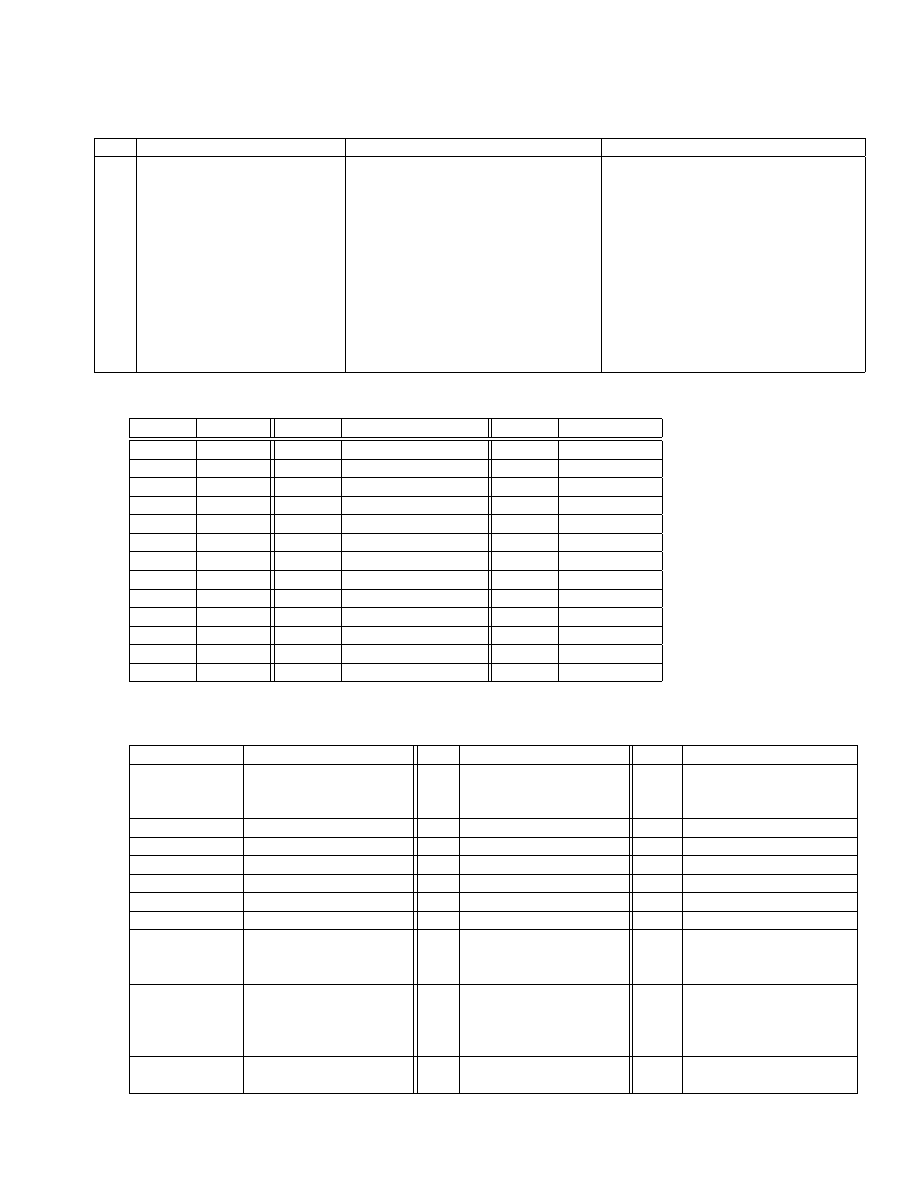
D. Hiebeler, Matlab / R Reference
32
No.
Description
Matlab
R
261
Build your own colormap us-
ing Red/Green/Blue triplets
Use an n × 3 matrix; each row
gives R,G,B intensities between 0
and 1. Can use as argument with
colormap. E.g. for 2 colors: mycmap
= [0.5 0.8 0.2 ; 0.2 0.2 0.7]
Use a vector of hexadecimal strings,
each beginning with ’#’ and giving
R,G,B intensities between 00 and FF.
E.g. c(’#80CC33’,’#3333B3’); can
use as argument to col= parameter
to image.
You can build such a
vector of strings from vectors of Red,
Green, and Blue intensities (each
between 0 and 1) as follows (for a
2-color example):
r=c(0.5,0.2);
g=c(0.8,0.2); b=c(0.2,0.7);
mycolors=rgb(r,g,b)
.
Matlab plotting specifications, for use with plot, fplot, semilogx, semilogy, loglog, etc:
Symbol
Color
Symbol
Marker
Symbol
Linestyle
b
blue
.
point (.)
-
solid line
g
green
o
circle (◦)
:
dotted line
r
red
x
cross (×)
-.
dash-dot line
c
cyan
+
plus sign (+)
--
dashed line
m
magenta
*
asterisk (∗)
y
yellow
s
square (¤)
k
black
d
diamond (♦)
w
white
v
triangle (down) (▽)
^
triangle (up) (△)
<
triangle (left) (⊳)
>
triangle (right) (⊲)
p
pentragram star
h
hexagram star
R plotting specifications for col (color), pch (plotting character), and type arguments, for use with plot,
matplot
, points, and lines:
col
Description
pch
Description
type
Description
’blue’
Blue
’a’
a (similarly for other
characters, but see ’.’
below for an exception
p
points
’green’
Green
19
solid circle
l
lines
’red’
Red
20
bullet (smaller circle)
b
both
’cyan’
Cyan
21
open circle
c
lines part only of “b”
’magenta’
Magenta
22
square
o
lines, points overplotted
’yellow’
Yellow
23
diamond
h
histogram-like lines
’black’
Black
24
triangle point-up
s
steps
’#RRGGBB’
hexadecimal specifica-
tion of Red, Green,
Blue
25
triangle point-down
S
another kind of steps
(Other names)
See colors() for list of
available color names.
’.’
rectangle of size 0.01
inch, 1 pixel, or 1 point
(1/72 inch) depending
on device
n
no plotting
(See table on next page
for more)
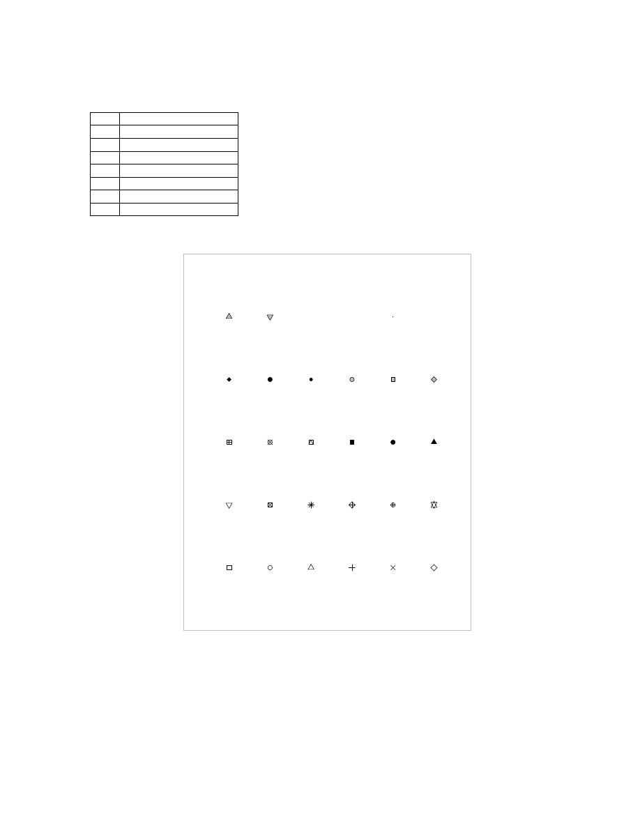
D. Hiebeler, Matlab / R Reference
33
R plotting specifications for lty (line-type) argument, for use with plot, matplot, points, and lines:
lty
Description
0
blank
1
solid
2
dashed
3
dotted
4
dotdash
5
longdash
6
twodash
0
1
2
3
4
5
6
7
8
9
10
11
12
13
14
15
16
17
18
19
20
21
22
23
24
25
A
A
b
b
.
#
#
R plotting characters, i.e. values for pch argument (from the book R Graphics, by Paul Murrell,
Chapman & Hall / CRC, 2006)

D. Hiebeler, Matlab / R Reference
34
No.
Description
Matlab
R
262
Divide up a figure window
into smaller sub-figures
subplot(m,n,k)
divides the current
figure window into an m × n ar-
ray of subplots, and draws in sub-
plot number k as numbered in “read-
ing order,” i.e. left-to-right, top-to-
bottom. E.g. subplot(2,3,4) se-
lects the first sub-figure in the second
row of a 2 × 3 array of sub-figures.
You can do more complex things,
e.g.
subplot(5,5,[1 2 6 7])
se-
lects the first two subplots in the first
row, and first two subplots in the
second row, i.e. gives you a bigger
subplot within a 5 × 5 array of sub-
plots. (If you that command followed
by e.g. subplot(5,5,3) you’ll see
what’s meant by that.)
There are several ways to do this, e.g.
using layout or split.screen, al-
though they aren’t quite as friendly
as Matlab ’s. E.g. if you let A =
1
1 2
1
1 3
4
5 6
, then layout(A) will
divide the figure into 6 sub-figures:
you can imagine the figure divide into
a 3 × 3 matrix of smaller blocks; sub-
figure 1 will take up the upper-left
2 × 2 portion, and sub-figures 2–6 will
take up smaller portions, according to
the positions of those numbers in the
matrix A. Consecutive plotting com-
mands will draw into successive sub-
figures; there doesn’t seem to be a way
to explicitly specify which sub-figure
to draw into next.
To
use
split.screen
,
you
can
do e.g.
split.screen(c(2,1))
to
split into a 2 × 1 matrix of sub-
figures (numbered 1 and 2).
Then
split.screen(c(1,3),2)
splits sub-
figure 2 into a 1 × 3 matrix of smaller
sub-figures (numbered 3, 4, and 5).
screen(4)
will then select sub-figure
number 4, and subsequent plotting
commands will draw into it.
A third way to accomplish this is
via the commands par(mfrow=) or
par(mfcol=)
to split the figure win-
dow, and par(mfg=) to select which
sub-figure to draw into.
Note that the above methods are all
incompatible with each other.
263
Force graphics windows to
update
drawnow
(Matlab normally only
updates figure windows when a
script/function finishes and returns
control to the Matlab prompt, or
under a couple of other circum-
stances.
This forces it to update
figure windows to reflect any recent
plotting commands.)
R automatically updates graphics
windows even before functions/scripts
finish executing, so it’s not neces-
sary to explictly request it. But note
that some graphics functions (partic-
ularly those in the lattice package)
don’t display their results when called
from scripts or functions; e.g. rather
than levelplot(...) you need to do
print(levelplot(...))
. Such func-
tions will automatically display their
plots when called interactively from
the command prompt.

D. Hiebeler, Matlab / R Reference
35
7.2
Printing/saving graphics
No.
Description
Matlab
R
264
To print/save to a PDF file
named fname.pdf
print -dpdf fname
saves the con-
tents of currently active figure win-
dow
First do pdf(’fname.pdf’). Then,
do
various
plotting
commands
to make your image,
as if you
were plotting in a window.
Fi-
nally, do dev.off() to close/save
the PDF file.
To print the con-
tents
of
the
active
figure
win-
dow,
do
dev.copy(device=pdf,
file=’fname.pdf’); dev.off()
.
(But this will not work if you’ve
turned
off
the
display
list
via
dev.control(displaylist=
’inhibit’)
.)
265
To print/save to a PostScript
file fname.ps or fname.eps
print -dps fname
for
black
&
white
PostScript;
print -dpsc
fname
for color PostScript; print
-deps fname
for black & white
Encapsulated
PostScript;
-depsc fname
for color Encapsu-
lated PostScript. The first two save
to fname.ps, while the latter two
save to fname.eps.
postscript(’fname.eps’)
, followed
by your plotting commands,
fol-
lowed by dev.off() to close/save
the file.
Note: you may want to
use
postscript(’fname.eps’,
horizontal=FALSE)
to save your fig-
ure in portrait mode rather than the
default landscape mode. To print the
contents of the active figure window,
do
dev.copy(device=postscript,
file=’fname.eps’); dev.off()
.
(But this will not work if you’ve
turned
off
the
display
list
via
dev.control(displaylist=
’inhibit’)
.) You can also include
the
horizontal=FALSE
argument
with dev.copy().
266
To print/save to a JPEG file
fname.jpg with jpeg qual-
ity = 90 (higher quality looks
better but makes the file
larger)
print -djpeg90 fname
jpeg(’fname.jpg’,quality=90)
,
followed by your plotting commands,
followed by dev.off() to close/save
the file.

D. Hiebeler, Matlab / R Reference
36
7.3
Animating cellular automata / lattice simulations
No.
Description
Matlab
R
267
To display images of cellu-
lar automata or other lattice
simulations while running in
real time
Repeatedly use either pcolor or
image
to display the data.
Don’t
forget to call drawnow as well, oth-
erwise the figure window will not be
updated with each image.
If you simply call image repeatedly,
there is a great deal of flicker-
ing/flashing.
To avoid this, after
drawing the image for the first time
using e.g.
image(A)
, from then
on only use image(A,add=TRUE),
which avoids redrawing the entire
image (and the associated flicker).
However, this will soon consume a
great deal of memory, as all drawn
images are saved in the image buffer.
There are two solutions to that
problem:
(1) every k time steps,
leave off the “add=TRUE” argument
to flush the image buffer (and get
occasional
flickering),
where
you
choose k to balance the flickering
vs.
memory-usage tradeoff;
or
(2) after drawing the first image,
do
dev.control(displaylist=
’inhibit’)
to prohibit retaining the
data.
However, the latter solution
means that after the simulation is
done, the figure window will not be
redrawn if it is resized, or temporarily
obscured by another window.
(A
call to dev.control(displaylist=
’enable’)
and
then
one
final
image(A)
at the end of the sim-
ulation
will
re-enable
re-drawing
after resizing or obscuring, without
consuming extra memory.)

D. Hiebeler, Matlab / R Reference
37
8
Working with files
No.
Description
Matlab
R
268
Create a folder (also known
as a “directory”)
mkdir dirname
dir.create(’dirname’)
269
Set/change working directory
cd dirname
setwd(’dirname’)
270
See list of files in current
working directory
dir
dir()
271
Run commands in file ‘foo.m’
or ‘foo.R’ respectively
foo
source(’foo.R’)
272
Read data from text file
“data.txt” into matrix A
A=load(’data.txt’)
or
A=importdata(’data.txt’)
Note
that both routines will ignore com-
ments (anything on a line following
a “%” character)
A=as.matrix(read.table(
’data.txt’))
This
will
ignore
comments
(anything
on
a
line
following a “#” character).
To ig-
nore comments indicated by “%”,
do
A=as.matrix(read.table(
’data.txt’, comment.char=’%’))
273
Write data from matrix A
into text file “data.txt”
save data.txt A -ascii
write(A, file=’data.txt’,
ncolumn=dim(A)[2])
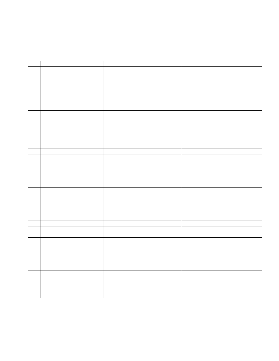
D. Hiebeler, Matlab / R Reference
38
9
Miscellaneous
9.1
Variables
No.
Description
Matlab
R
274
Assigning to variables
x = 5
x <- 5
or x = 5 Note: for compati-
bility with S-plus, many people prefer
the first form.
275
From within a function, as-
sign a value to variable y
in the base environment (i.e.
the command prompt envi-
ronment)
assignin(’base’, ’y’, 7)
y <<- 7
276
From within a function, ac-
cess the value of variable y
in the base environment (i.e.
the command prompt envi-
ronment)
evalin(’base’, ’y’)
get(’y’, envir=globalenv())
Though note that inside a function,
if there isn’t a local variable y, then
just the expression y will look for one
in the base environment, but if there
is a local y then that one will be used
instead.
277
Short list of defined variables
who
ls()
278
Long list of defined variables
whos
ls.str()
279
See detailed info about the
variable ab
whos ab
str(ab)
280
See detailed info about all
variables with “ab” in their
name
whos *ab*
ls.str(pattern=’ab’)
281
Open graphical data editor,
to edit the value of variable
A (useful for editing values in
a matrix, though it works for
non-matrix variables as well)
openvar(A)
, or double-click on the
variable in the Workspace pane (if
it’s being displayed) of your Mat-
labdesktop
fix(A)
282
Clear one variable
clear x
rm(x)
283
Clear two variables
clear x y
rm(x,y)
284
Clear all variables
clear all
rm(list=ls())
285
See what type of object x is
class(x)
class(x)
286
(Variable names)
Variable names must begin with a
letter, but after that they may con-
tain any combination of letters, dig-
its, and the underscore character.
Names are case-sensitive.
Variable names may contain letters,
digits, the period, and the underscore
character. They cannot begin with a
digit or underscore, or with a period
followed by a digit. Names are case-
sensitive.
287
Result of last command
ans
contains the result of the last
command which did not assign its
value to a variable. E.g. after 2+5;
x=3
, then ans will contain 7.
.Last.value
contains the result of
the last command, whether or not its
value was assigned to a variable. E.g.
after 2+5; x=3, then .Last.value will
contain 3.

D. Hiebeler, Matlab / R Reference
39
9.2
Strings and Misc.
No.
Description
Matlab
R
288
Line continuation
If you want to break up a Matlab
command over more than one line,
end all but the last line with three
periods: “...”. E.g.:
x = 3 + ...
4
or
x = 3 ...
+ 4
In R, you can spread commands out
over multiple lines, and nothing ex-
tra is necessary. R will continue read-
ing input until the command is com-
plete. However, this only works when
the syntax makes it clear that the first
line was not complete. E.g.:
x = 3 +
4
works, but
x = 3
+ 4
does not treat the second line as a con-
tinuation of the first.
289
Controlling
formatting
of
output
format short g
and
format long g
are
handy;
see
help format
options(digits=6)
tells R you’d like
to use 6 digits of precision in values it
displays (it is only a suggestion, not
strictly followed)
290
Exit the program
quit
or exit
q()
or quit()
291
Comments
% this is a comment
# this is a comment
292
Display a string
disp(’hi there’)
or
to
omit
trailing
newline
use
fprintf(’hi there’)
print(’hi there’)
293
Display a string containing
single quotes
disp(’It’’s nice’)
or
to
omit
trailing
newline
fprintf(’It’’s nice’)
print(’It\’s nice’)
or
print("It’s nice")
294
Give prompt and read numer-
ical input from user
x = input(’Enter data:’)
print(’Enter data:’); x=scan()
But note: if in a script and you use
the Edit → Execute menu item to
run it, the selected text after the
scan statement will be used as source
for the input, rather than keyboard.
295
Give prompt and read char-
acter (string) input from user
x = input(’Enter string:’,’s’)
x = readline(’Enter string:’)
296
Concatenate strings
[’two hal’ ’ves’]
paste(’two hal’, ’ves’, sep=’’)
297
Concatenate strings stored in
a vector
v={’two ’, ’halves’};
strcat(v{:})
But
note
that
this
drops
trailing
spaces
on
strings. To avoid that, instead do
strcat([v{:}])
v=c(’two ’, ’halves’);
paste(v, collapse=’’)
298
Extract substring of a string
text1=’hi there’;
text2=text(2:6)
text1=’hi there’;
text2=substr(text1,2,6)
299
Determine whether elements
of a vector are in a set, and
give positions of correspond-
ing elements in the set.
x = {’a’, ’aa’, ’bc’, ’c’}; y
= {’da’, ’a’, ’bc’, ’a’, ’bc’,
’aa’}; [tf, loc]=ismember(x,y)
Then loc contains the locations of
last
occurrences of elements of x
in the set y, and 0 for unmatched
elements.
x = c(’a’, ’aa’, ’bc’, ’c’); y
= c(’da’, ’a’, ’bc’, ’a’, ’bc’,
’aa’); loc=match(x,y)
Then loc
contains the locations of first oc-
curences of elements of x in the set
y, and NA for unmatched elements.

D. Hiebeler, Matlab / R Reference
40
No.
Description
Matlab
R
300
Convert number to string
num2str(x)
as.character(x)
301
Use sprintf to create a
formatted string. Use %d for
integers (“d” stands for “dec-
imal”, i.e. base 10), %f for
floating-point numbers, %e
for scientific-notation floating
point, %g to automatically
choose %e or %f based on
the value.
You can spec-
ify
field-widths/precisions,
e.g.
%5d for integers with
padding to 5 spaces, or %.7f
for
floating-point
with
7
digits of precision. There are
many other options too; see
the docs.
x=2; y=3.5;
s=sprintf(’x is %d, y=%g’, ...
x, y)
x=2; y=3.5
s=sprintf(’x is %d, y is %g’,
x, y)
302
Machine epsilon ǫ
mach
, i.e.
difference between 1 and the
next largest double-precision
floating-point number
eps
(See help eps for various other
things eps can give.)
.Machine$double.eps
303
Pause for x seconds
pause(x)
Sys.sleep(x)
304
Wait for user to press any key
pause
Don’t know of a way to do this in R,
but scan(quiet=TRUE) will wait until
the user presses the Enter key
305
Measure CPU time used to
do some commands
t1=cputime; ...commands...
;
cputime-t1
t1=proc.time(); ...commands...
; (proc.time()-t1)[1]
306
Measure
elapsed
(“wall-
clock”) time used to do some
commands
tic; ...commands...
; toc
or
t1=clock; ...commands...
;
etime(clock,t1)
t1=proc.time(); ...commands...
; (proc.time()-t1)[3]
307
Print an error message an in-
terrupt execution
error(’Problem!’)
stop(’Problem!’)
308
Print a warning message
warning(’Smaller problem!’)
warning(’Smaller problem!’)
309
Putting multiple statements
on one line
Separate statements by commas or
semicolons. A semicolon at the end
of a statement suppresses display of
the results (also useful even with just
a single statement on a line), while a
comma does not.
Separate statements by semicolons.
310
Evaluate contents of a string
s as command(s).
eval(s)
eval(parse(text=s))
311
Get a command prompt for
debugging, while executing a
script or function. While at
that prompt, you can type ex-
pressions to see the values of
variables, etc.
Insert the command keyboard in
your file. Note that your prompt will
change to K>>. When you are done
debugging and want to continue ex-
ecuting the file, type return.
Insert the command browser() in
your file. Note that your prompt will
change to Browse[1]>. When you are
done debugging and want to continue
executing the file, either type c or just
press return (i.e. enter a blank line).
Note, if you type n, you enter the step
debugger.

D. Hiebeler, Matlab / R Reference
41
No.
Description
Matlab
R
312
Show where a command is
which sqrt
shows you where the file
defining the sqrt function is (but
note that many basic functions are
“built in,” so the Matlab func-
tion file is really just a stub con-
taining documentation). This is use-
ful if a command is doing something
strange, e.g. sqrt isn’t working. If
you’ve accidentally defined a variable
called sqrt, then which sqrt will
tell you, so you can clear sqrt to
erase it so that you can go back to
using the function sqrt.
R does not execute commands directly
from files, so there is no equivalent
command.
313
Query/set the search path.
path
displays the current search path
(the list of places Matlab searches
for commands you enter). To add a
directory ~/foo to the beginning of
the search path, do
addpath ~/foo -begin
or to add it to the end of the path,
do addpath ~/foo -end (Note: you
should generally add the full path
of a directory, i.e. in Linux or Mac
OS-X something like ~/foo as above
or of the form /usr/local/lib/foo,
while under Windows it would be
something like C:/foo)
R does not use a search path to look
for files.
314
Startup sequence
If a file startup.m exists in the
startup directory for Matlab, its
contents are executed.
(See the
Matlab docs for how to change the
startup directory.)
If a file .Rprofile exists in the cur-
rent directory or the user’s home di-
rectory (in that order), its contents
are sourced; saved data from the file
.RData (if it exists) are then loaded.
If a function .First() has been de-
fined, it is then called (so the obvious
place to define this function is in your
.Rprofile file).
315
Shutdown sequence
Upon typing quit or exit, Matlab
will run the script finish.m if present
somewhere in the search path.
Upon typing q() or quit(), R will call
the function .Last() if it has been de-
fined (one obvious place to define it
would be in the .Rprofile file)

D. Hiebeler, Matlab / R Reference
42
No.
Description
Matlab
R
316
Install and load a package.
Matlab does not have packages. It
has toolboxes, which you can pur-
chase and install.
“Contributed”
code (written by end users) can sim-
ply be downloaded and put in a di-
rectory which you then add to Mat-
lab’s path (see item 313 for how to
add things to Matlab’s path).
To install e.g.
the deSolve pack-
age,
you can use the command
install.packages(’deSolve’)
.
You then need to load the package
in order to use it, via the command
library(’deSolve’)
. When running
R again later you’ll need to load the
package again to use it, but you
should not need to re-install it. Note
that the lattice package is typically
included with binary distributions of
R, so it only needs to be loaded, not
installed.
10
Spatial Modeling
No.
Description
Matlab
R
317
Take an L×L matrix A of
0s and 1s, and “seed” frac-
tion p of the 0s (turn them
into 1s), not changing entries
which are already 1.
A = (A | (rand(L) < p))*1;
A = (A | (matrix(runif(L^2),L)
< p))*1
318
Take an L × L matrix A of 0s
and 1s, and “kill” fraction p
of the 1s (turn them into 0s),
not changing the rest of the
entries
A = (A & (rand(L) < 1-p))*1;
A = (A & (matrix(runif(L^2),L)
< 1-p))*1
319
Do “wraparound” on a coor-
dinate newx that you’ve al-
ready calculated.
You can
replace newx with x+dx if
you want to do wraparound
on an offset x coordinate.
mod(newx-1,L)+1
Note: for porta-
bility with other languages such as
C which handle MOD of negative
values differently, you may want to
get in the habit of instead doing
mod(newx-1+L,L)+1
((newx-1) %% L) + 1
Note:
for
portability with other languages such
as C which handle MOD of nega-
tive values differently, you may want
to get in the habit of instead doing
((newx-1+L)%%L) + 1
320
Randomly initialize a portion
of an array: set fraction p of
sites in rows iy1 through iy2
and columns ix1 through ix2
equal to 1 (and set the rest of
the sites in that block equal
to zero). Note: this assume
iy1 < iy2 and ix1 < ix2.
dx=ix2-ix1+1; dy=iy2-iy1+1;
A(iy1:iy2,ix1:ix2) = ...
(rand(dy,dx) < p0)*1;
dx=ix2-ix1+1; dy=iy2-iy1+1;
A[iy1:iy2,ix1:ix2] =
(matrix(runif(dy*dx),dy) <
p0)*1

INDEX OF MATLAB COMMANDS AND CONCEPTS
43
Index of MATLAB commands and concepts
’
, 77
,
, 309
.*
, 76
...
, 288
./
, 82
.^
, 86
/
, 81
:
, 12–14
;
, 309
=
, 274
[
, 6–8
%
, 291
&
, 175, 176
^
, 50, 84, 85
\
, 78, 83
{
45
abs
, 51, 70
acos
, 56
acosh
, 58
addpath
, 313
all
, 177
angle
, 71
annotation
, 252, 253
ans
, 287
any
, 178
arrows in plots, 252, 253
asin
, 56
asinh
, 58
assignin
, 275
atan
, 56
atanh
, 58
average, see mean
axis
, 244
bar
, 233, 235, 236
binocdf
, 218
binopdf
, 211
binornd
, 202
boolean tests
scalar, 175
vector, 176–178
break
, 180
cd
, 269
ceil
, 62
cell
, 44
cell arrays, 44
extracting elements of, 45
cellular automata animation, 267
chol
, 92
class
, 285
clear
, 282–284
clf
, 255
clock
, 306
close
, 228
colon, see :
colorbar
, 259
colormap
building your own, 261
colormap
, 260, 261
column vector, 7
comments, 291
complex numbers, 69–74
cond
, 96–98
conj
, 72
continue
, 180
contour
, 243
conv
, 154
corr
, 110–115
cos
, 55
cosh
, 57
cov
, 108, 109
cputime
, 305
csape
, 167, 169, 170
cubic splines, 168, 169
natural, 167
not-a-knot, 171
periodic, 170
cumprod
, 124
cumsum
, 120–123
cumulative distribution functions
binomial, 218
continuous uniform on interval (a, b), 222
discrete uniform from 1..n, 223
exponential, 220
normal, 221
Poisson, 219
debugging, 311
diag
, 22, 23
diff
, 126
differential equations, see ode45
dir
, 270
disp
, 292, 293
doc
, 4
drawnow
, 263, 267
echelon form, see matrix
eig
, 88

INDEX OF MATLAB COMMANDS AND CONCEPTS
44
element-by-element matrix operations, see ma-
trix
else
, 174
elseif
, 174
end
, 36
eps
, 302
erf
, 64
erfc
, 65
erfcinv
, 67
erfinv
, 66
error
, 307
errorbar
, 237, 238
etime
, 306
eval
, 310
evalin
, 276
exit
, 290
exp
, 52
expcdf
, 220
expm
, 119
exppdf
, 213
exprnd
, 204
eye
, 21
figure
, 224, 225
file
reading data from, 273
running commands in, 271
text
reading data from, 272
saving data to, 273
find
, 149–151
finish.m, 315
floor
, 61
fminbnd
, 157, 158
fminsearch
, 159, 160
font size in plots, 248
for
, 172
format
, 289
fplot
, 257
fprintf
, 292, 293
function
multi-variable
minimization, 159
minimization over first parameter only, 158
minimization over only some parameters,
160
single-variable
minimization, 157
user-written, 182
returning multiple values, 183
fzero
, 156
gca
, 248
gcf
, 226
get
, 227
Greek letters
in plot labels, 247
grid
, 249
help
, 1–3
helpbrowser
, 4
helpdesk
, 4
hilb
, 42
hist
, 152, 153, 234, 235
hold
, 255
identity, see matrix
if
, 173–175
imag
, 74
image
, 258, 267
imagesc
, 258
importdata
, 272
ind2sub
, 32
indexing
matrix, 10
with a single index, 11
vector, 9
input
, 294, 295
inv
, 80
inverse, see matrix
ismember
, 299
keyboard
, 311
legend
, 254
length
, 139, 141
linspace
, 15
load
, 272, 273
log
, 53
log10
, 54
log2
, 54
loglog
, 232
logspace
, 16
lookfor
, 5
lu
, 89
matrix, 8
boolean operations on, 150, 151
changing shape of, 39
Cholesky factorization, 92
condition number, 96–98
containing all indentical entries, 20
containing all zeros, 19
converting row, column to single index, 33
converting single-index to row, column, 32
cumulative sums of all elements of, 123
cumulative sums of columns, 121

INDEX OF MATLAB COMMANDS AND CONCEPTS
45
cumulative sums of rows, 122
diagonal, 22
echelon form, 79
eigenvalues and eigenvectors of, 88
equation
solving, 78
exponential of, 119
extracting a column of, 27
extracting a rectangular piece of, 30
extracting a row of, 28
extracting specified rows and columns of, 31
“gluing” together, 24, 25
identity, 21
inverse, 80
lower-triangular portion of, 40
LU factorization, 89
minimum of values of, 129
minimum value of each column of, 130
minimum value of each row of, 131
modifying elements given lists of rows and
columns, 34
multiplication, 75
element-by-element, 76
N -dimensional, 43
norm, 95
powers of, 85
QR factorization, 93
rank, 87
re-shaping its elements into a vector, 29
Schur decomposition, 91
singular value decomposition, 90
size of, 136–138, 140, 141
sum
of all elements, 116
of columns of, 117
of rows of, 118
transpose, 77
upper-triangular portion of, 41
max, see min
mean
, 99–101
mesh
, 243
meshgrid
, 110, 242
min
, 128–131, 133–135
mind
, 132
mkdir
, 268
mnpdf
, 217
mnrnd
, 209, 210
mod
, 59, 319
modulo arithmetic, 59, 319
multiple statements on one line, 309
nchoosek
, 68
norm
, 94, 95
normcdf
, 221
normpdf
, 214
normrnd
, 208
num2str
, 300
numel
, 140
ode45
, 184–186
ones
, 18, 20
openvar
, 281
optimization, 157–160
path
, 313
pause
, 303, 304
pcolor
, 243, 258, 267
perform some commands with probability p, 196
permutation of integers 1..n, 197
plot
, 229–231, 256
Greek letters in axis labels, 247
plot3
, 240
poisscdf
, 219
poisspdf
, 212
poissrnd
, 203
polar
, 239
polyfit
, 163–165
polynomial
least-squares fitted, 164–166
multiplication, 154
roots of, 155
ppval
, 167, 169, 170
, 264–266
probability density functions
binomial, 211
continuous uniform on interval (a, b), 215
discrete uniform from 1..n, 216
exponential, 213
multinomial, 217
normal, 214
Poisson, 212
qr
, 93
quad
, 161
quit
, 290
rand
, 187–195, 201
random values
Bernoulli, 193
binomial, 202
continuous uniform distribution on interval
(a, b), 190, 207
continuous uniform distribution on interval
(0,1), 187–189
discrete uniform distribution from a..b, 195
discrete uniform distribution from 1..k, 192,
205, 206

INDEX OF MATLAB COMMANDS AND CONCEPTS
46
discrete uniform distribution, 191
exponential, 204
k unique values sampled from integers 1..n,
198
multinomial, 209, 210
normal, 208
Poisson, 203
setting the seed, 201
randperm
, 197, 198
randsample
, 198–200
rank
, 87
rcond
, 96
real
, 73
reshape
, 39, 43
roots
of general single-variable function, 156
polynomial, 155
roots
, 155
round
, 60
row vector, 6
rref
, 79
sampling values from a vector, 199, 200
save
, 273
schur
, 91
semilogx
, 232
semilogy
, 232
set
, 248
shading
, 258
sign
, 63
sin
, 55
sinh
, 57
size
, 136–138
slice
, 243
sort
, 142, 143, 198
sortrows
, 144–147
spline
, 171
splines, see cubic splines
sprintf
, 301
sqrt
, 49
stairs
, 239
standard deviation, see std
startup.m, 314
std
, 102–104
stem
, 239
stop
, 307
strcat
, 297
string
concatenation, 296
converting number to, 300
substrings, 298
struct
, 47
sub2ind
, 33, 34
subplot
, 262
sum
, 116–118, 176
surf
, 241, 242
surfc
, 243
surfl
, 243
svd
, 90
switch
, 181
tan
, 55
tanh
, 57
text
, 250, 251
tic
, 306
title
, 245
toc
, 306
transpose, see matrix
trapz
, 162
tril
, 40
triu
, 41
unidcdf
, 223
unidpdf
, 216
unidrnd
, 205, 206
unifcdf
, 222
unifpdf
, 215
unifrnd
, 207
unique
, 152, 235
var
, 105–107
variables
assigning, 274
assigning in base environment from func-
tion, 275
evaluating from base environment within func-
tion, 276
names, 286
variance, see var
vector
boolean operations on, 148, 149
containing all indentical entries, 18
containing all zeros, 17
counts of binned values in, 153
counts of discrete values in, 152
cumulative sum of elements of, 120
differences between consecutive elements of,
126
minimum of values of, 128
norm, 94
position of first occurance of minimum value
in, 135
reversing order of elements in, 26
size of, 139
sum of all elements, 116
truncating, 35

INDEX OF MATLAB COMMANDS AND CONCEPTS
47
warning
, 308
waterfall
, 243
which
, 312
while
, 179
who
, 277
whos
, 278–280
xlabel
, 246–248
ylabel
, 246, 247
zeros
, 17, 19

INDEX OF R COMMANDS AND CONCEPTS
48
Index of R commands and concepts
*
, 84
/
, 82
:
, 12, 13
;
, 309
<-
, 274
<<-
, 275
=
, 274
?
, 1, 2
[[
, 45
#
, 291
%%
, 59, 319
&
, 175, 176
^
, 50, 86
abs
, 51, 70
acos
, 56
acosh
, 58
all
, 177
any
, 178
apply
, 104, 106, 107, 130, 131
Arg
, 71
array
, 43
arrows
, 252, 253
as.character
, 300
as.numeric
, 152
asin
, 56
asinh
, 58
atan
, 56
atanh
, 58
average, see mean
barplot
, 233, 235
boolean tests
scalar, 175
vector, 176–178
break
, 180
browser
, 311
c
, 6, 7
cbind
, 24, 34
ceiling
, 62
cellular automata animation, 267
chol
, 92
choose
, 68
class
, 285
cloud
, 240
coef
, 163, 164, 166
colMeans
, 100
colon, see :
colormap
building your own, 261
for image, 260
colSums
, 117
column vector, 7
comments, 291
complex numbers, 69–74
Conj
, 72
contour
, 243
convolve
, 154
cor
, 111–115
cos
, 55
cosh
, 57
cov
, 108–110
cubic splines, 168, 169, 171
natural, 167
periodic, 170
cummax
, 125
cummin
, 125
cumprod
, 124
cumsum
, 120–123
cumulative distribution functions
binomial, 218
continuous uniform on interval (a, b), 222
discrete uniform from 1..n, 223
exponential, 220
normal, 221
Poisson, 219
curve
, 257
data.frame
, 47
dbinom
, 211
debugging, 311
dev.control
, 264, 265, 267
dev.copy
, 264, 265
dev.cur()
, 226
dev.list
, 227
dev.new
, 224
dev.off
, 228, 264–266
dev.set
, 225
dexp
, 213
diag
, 21–23
diff
, 126
differential equations, see lsoda
dim
, 39, 138, 141
dir
, 270
dir.create
, 268
dmultinom
, 217
dnorm
, 214
dpois
, 212
dunif
, 215

INDEX OF R COMMANDS AND CONCEPTS
49
echelon form, see matrix
eig
, 88
element-by-element matrix operations, see ma-
trix
else
, 174
errbar
, 237, 238
eval
, 310
exp
, 52
expand
, 89
expand.grid
, 243
expm
, 119
file
reading data from, 273
running commands in, 271
text
reading data from, 272
saving data to, 273
filled.contour
, 259
.First
, 314
fix
, 281
floor
, 61
font size in plots, 248
for
, 172
function
multi-variable
minimization, 159
minimization over first parameter only, 158
minimization over only some parameters,
160
single-variable
minimization, 157
user-written, 182
returning multiple values, 183
get
, 276
globalenv
, 276
graphics
not being displayed from scripts/functions,
263
Greek letters
in plot labels, 247
grid
, 249
help
, 1, 2
help.search
, 5
help.start
, 4
Hilbert
, 42
hist
, 153, 233, 234, 236
identity, see matrix
if
, 173–175
ifelse
, 127
Im
, 74
image
, 258, 267
indexing
matrix, 10
with a single index, 11
vector, 9
install.packages
, 316
integrate
, 161
inverse, see matrix
jpeg
, 266
kappa
, 97
.Last
, 315
.Last.value
, 287
lattice package, 243, 259, 263, 316
layout
, 262
legend
, 254
length
, 35, 36, 139, 140
levelplot
, 259, 263
library
, 3, 316
lines
, 255
lists, 44
extracting elements of, 45
lm
, 163, 164, 166
log
, 53
log10
, 54
log2
, 54
lower.tri
, 41
ls
, 277
ls.str
, 278, 280
lsoda
, 184–186
.Machine$double.eps
, 302
match
, 299
matplot
, 256
matrix, 8
boolean operations on, 150, 151
changing shape of, 39
Cholesky factorization, 92
condition number, 96–98
containing all indentical entries, 20
containing all zeros, 19
converting row, column to single index, 33
converting single-index to row, column, 32
cumulative sums of all elements of, 123
cumulative sums of columns, 121
cumulative sums of rows, 122
diagonal, 22
echelon form, 79
eigenvalues and eigenvectors of, 88
equation
solving, 78
exponential of, 119

INDEX OF R COMMANDS AND CONCEPTS
50
extracting a column of, 27
extracting a rectangular piece of, 30
extracting a row of, 28
extracting specified rows and columns of, 31
“gluing” together, 24, 25
identity, 21
inverse, 80
lower-triangular portion of, 40
LU factorization, 89
minimum of values of, 129
minimum value of each column of, 130
minimum value of each row of, 131
modifying elements given lists of rows and
columns, 34
multiplication, 75
element-by-element, 76
N -dimensional, 43
norm, 95
powers of, 85
QR factorization, 93
rank, 87
re-shaping its elements into a vector, 29
Schur decomposition, 91
singular value decomposition, 90
size of, 136–138, 140, 141
sum
of all elements, 116
of columns of, 117
of rows of, 118
transpose, 77
upper-triangular portion of, 41
matrix
, 8, 19, 20
max, see min
mean
, 99
min
, 128–131, 134
Mod
, 70
modulo arithmetic, 59, 319
multiple statements on one line, 309
names
, 46, 152
ncol
, 137
next
, 180
norm
, 94, 95
nrow
, 136
optim
, 159, 160
optimization, 157–160
optimize
, 157, 158
options
digits=
, 289
order
, 144–147
outer
, 242
packages
installing, 316
loading, 316
par
, 248
par
mfcol=
, 262
mfrow=
, 262
parse
, 310
paste
, 296, 297
pbinom
, 218
, 248, 264
perform some commands with probability p, 196
permutation of integers 1..n, 197
persp
, 241, 242
pexp
, 220
pie
, 239
plot
, 229–232
Greek letters in axis labels, 247
main=
, 245
sub=
, 245
xlab=
, 246, 247
xlim=
, 244
ylab=
, 246, 247
ylim=
, 244
pmin
, 132, 133
pnorm
, 64, 65, 221
points
, 255
polynomial
least-squares fitted, 164–166
multiplication, 154
roots of, 155
polyreg
, 165
polyroot
, 155
postscript
, 265
ppois
, 219
, 263, 292, 293
probability density functions
binomial, 211
continuous uniform on interval (a, b), 215
discrete uniform from 1..n, 216
exponential, 213
multinomial, 217
normal, 214
Poisson, 212
proc.time
, 305, 306
punif
, 222
q
, 290
qnorm
, 66, 67
qr
, 87, 93
quartz
, 224
quit
, 290
rand
, 194

INDEX OF R COMMANDS AND CONCEPTS
51
random values
Bernoulli, 193
binomial, 202
continuous uniform distribution on interval
(a, b), 190, 207
continuous uniform distribution on interval
(0,1), 187, 189
continuous uniform distribution on inteval
(0,1), 188
discrete uniform distribution from a..b, 195
discrete uniform distribution from 1..k, 192,
205, 206
discrete uniform distribution, 191
exponential, 204
k unique values sampled from integers 1..n,
198
multinomial, 209, 210
normal, 208
Poisson, 203
setting the seed, 201
rbind
, 25
rbinom
, 202
rcond
, 96, 98
.RData
, 314
Re
, 73
read.table
, 272, 273
readline
, 295
rep
, 17, 18
rev
, 26
rexp
, 204
rgb
, 261
rm
, 282–284
rmultinom
, 209, 210
rnorm
, 208
roots
of general single-variable function, 156
polynomial, 155
round
, 60
row vector, 6
rowMeans
, 101
rpois
, 203
.Rprofile
, 314
runif
, 187–193, 195, 207
sample
, 197–200, 205, 206
sampling values from a vector, 199, 200
scan
, 294, 304
Schur
, 91
sd
, 102–104
seq
, 14–16
set.seed
, 201
setwd
, 269
sign
, 63
sin
, 55
sinh
, 57
solve
, 78, 80, 81, 83
sort
, 142, 143
source
, 271
spline
, 167, 168, 170
splines, see cubic splines
split.screen
, 262
sprintf
, 301
sqrt
, 49
standard deviation, see sd
str
, 279
string
concatenation, 296
converting number to, 300
substrings, 298
substr
, 298
sum
, 116, 118, 176
svd
, 90
switch
, 181
symbols
, 243
Sys.sleep
, 303
t
, 77
table
, 152, 235
tan
, 55
tanh
, 57
text
, 250, 251
title
, 245, 246
transpose, see matrix
uniroot
, 156
upper.tri
, 40
var
, 105–107, 109
variables
assigning, 274
assigning in base environment from func-
tion, 275
evaluating from base environment within func-
tion, 276
names, 286
variance, see var
vector
boolean operations on, 148, 149
containing all indentical entries, 18
containing all zeros, 17
counts of binned values in, 153
counts of discrete values in, 152
cumulative sum of elements of, 120
differences between consecutive elements of,
126
minimum of values of, 128
norm, 94

INDEX OF R COMMANDS AND CONCEPTS
52
position of first occurance of minimum value
in, 135
reversing order of elements in, 26
size of, 139
sum of all elements, 116
truncating, 35
vector
, 44
warning
, 308
which
, 149–151
which.max
, see which.min
which.min
, 135
while
, 179
windows
, 224
wireframe
, 243
write
, 273
x11
, 224
Wyszukiwarka
Podobne podstrony:
Matlab1 4 id 287787 Nieznany
MATLAB~3 id 287655 Nieznany
matlab3 id 287802 Nieznany
Matlab intro id 287680 Nieznany
MATLAB cw 2 id 287670 Nieznany
MATLAB cwiczenia cwmatl id 2876 Nieznany
konspekt Matlab 2012 id 245613 Nieznany
LAB1 MES MATLAB statyka 1 id 25 Nieznany
MATLAB AMGd wprowadzenie id 287 Nieznany
przetwrzanie obrazw matlab id 4 Nieznany
MATLAB rozdzial5 id 768819 Nieznany
matlab Komendy id 287424 Nieznany
pinf13 matlab cz3 id 358238 Nieznany
MATLAB cw 09 11 Wykresy id 2876 Nieznany
Abolicja podatkowa id 50334 Nieznany (2)
4 LIDER MENEDZER id 37733 Nieznany (2)
katechezy MB id 233498 Nieznany
metro sciaga id 296943 Nieznany
więcej podobnych podstron