Track A – NI Data Acqusion with Microphone:
USB-6009 with Microphone & LED
Suggested Hardware:
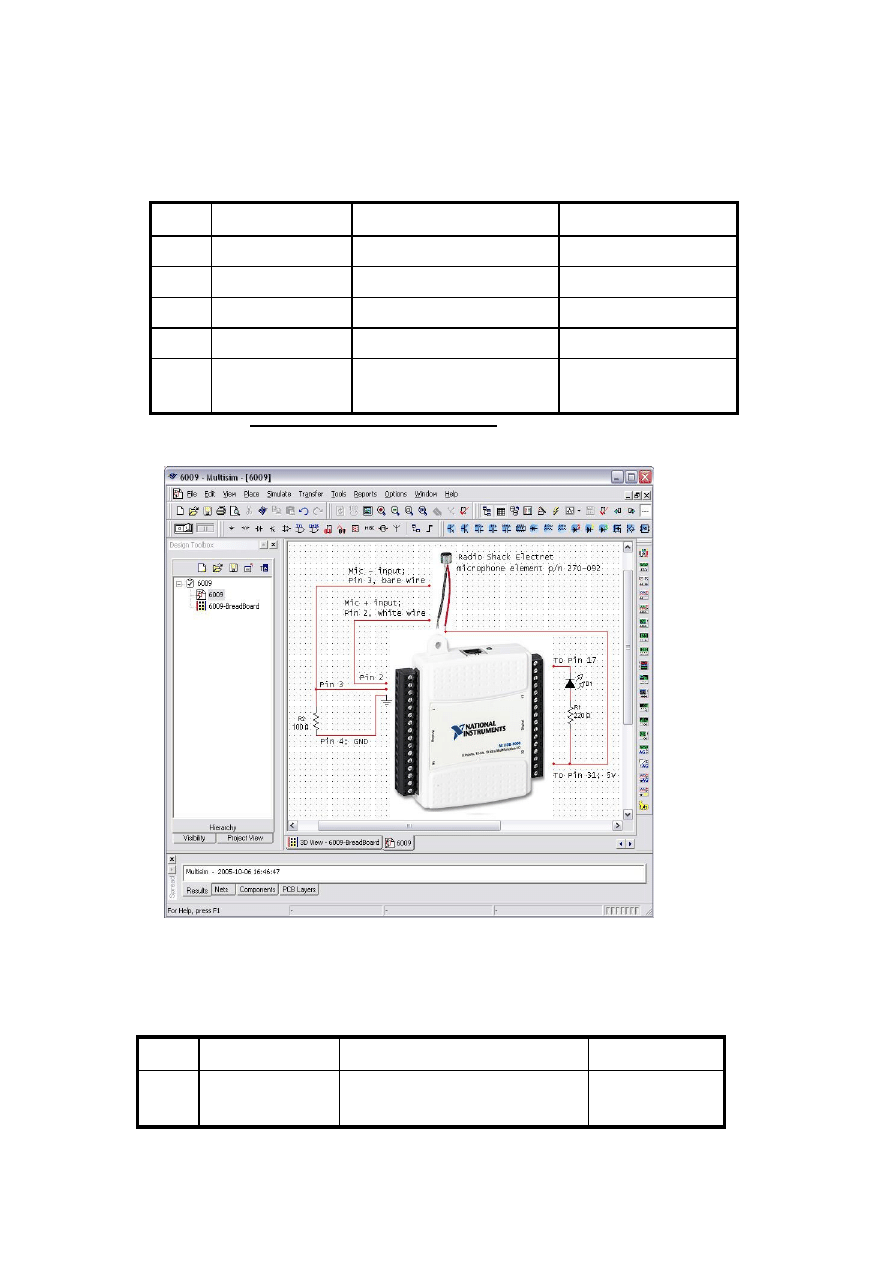
The following schematic was drawn with Multisim, a widely used SPICE schematic capture and
simulation tool. Visit http://www.electronicsworkbench.com for more info.
Setting-Up Your Hardware for Your Selected Track
RadioShack
220 Ohm Resistor
1
RadioShack
Electret Microphone
270-092
1
RadioShack
100 Ohm Resistor
1
RadioShack
Light Emitting Diode
(LED)
276-307
1
National Instruments
Low-cost USB DAQ
779321-22
1
Supplier
Description
Part Number
Qty
Track B – Simulated NI Data Acqusion:
NI-DAQ Software version 8.0 or newer
Track C – Third-party Soundcard:
Soundcard and Microphone
Suggested Hardware:
* Laptops often have a built-in microphone (no plug-in microphone is required)
RadioShack
Standard Plug-in PC
Microphone*
1
Supplier
Description
Part Number
Qty

Exercise 1.1 – Testing Your Device (Track A)
In this exercise you will use Measurement and Automation Explorer (MAX) to test
your NI USB-6009 DAQ device.
1. Launch MAX by double-clicking the icon on the desktop or by selecting
Start»Programs»National Instruments»Measurement & Automation.
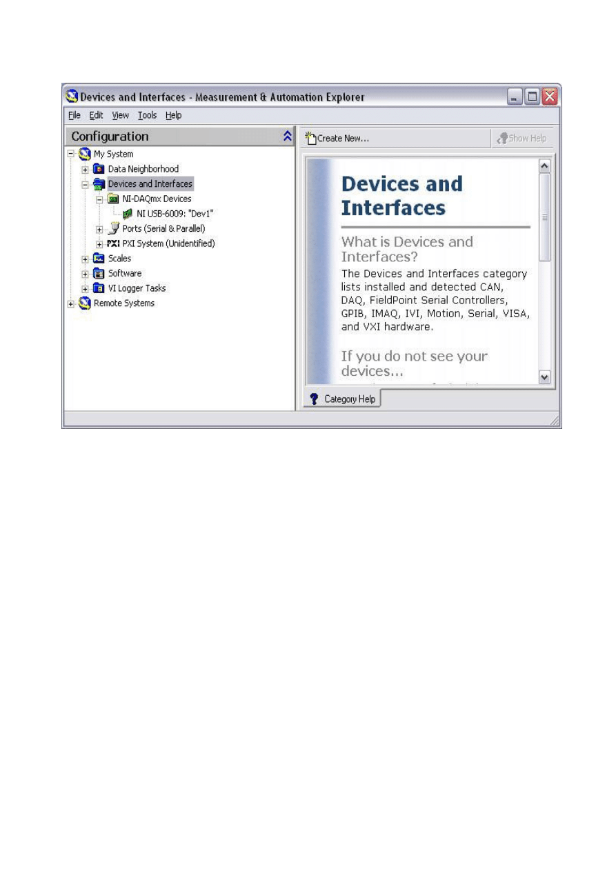
2. Expand the Devices and Interfaces section to view the installed National
Instruments devices. MAX displays the National Instruments hardware and software
in the computer.
3. Expand the NI-DAQmx Devices section to view the installed hardware that is
compatible with NI-DAQmx. The device number appears in quotes following the
device name. The data acquisition VIs use this device number to determine which
device performs DAQ operations. You will see your hardware listed as NI USB-
6009: “Dev1”.
4. Perform a self-test on the device by right-clicking it in the configuration tree and
choosing Self-Test or clicking “Self-Test” along the top of the window. This tests the
system resources assigned to the device. The device should pass the test because it is
already configured.
5. Check the pinout for your device. Right-click the device in the configuration tree and
select Device Pinouts or click “Device Pinouts” along the top of the center window.
6. Open the test panels. Right-click the device in the configuration tree and select Test
Panels… or click “Test Panels…” along the top of the center window. The test
panels allow you to test the available functionality of your device, analog
input/output, digital input/output, and counter input/output without doing any
programming.
7. On the Analog Input tab of the test panels, change Mode to “Continuous” and Rate
to 10,000 Hz. Click “Start” and hum or whistle into your microphone to observe the
signal that is plotted. Click “Finish” when you are done.
8. On the Digital I/O tab notice that initially the port is configured to be all input.
Observe under Select State the LEDs that represent the state of the input lines. Click
the “All Output” button under Select Direction. Notice you now have switches under
Select State to specify the output state of the different lines. Toggle line 0 and watch
the LED light up. Click “Close” to close the test panels.
9. Close MAX.
(End of Exercise)

Exercise 1.1 – Setting Up Your Device (Track B)
In this exercise you will use Measurement and Automation Explorer (MAX) to configure
a simulated DAQ device.
1. Launch MAX by double-clicking the icon on the desktop or by selecting
Start»Programs»National Instruments»Measurement & Automation.
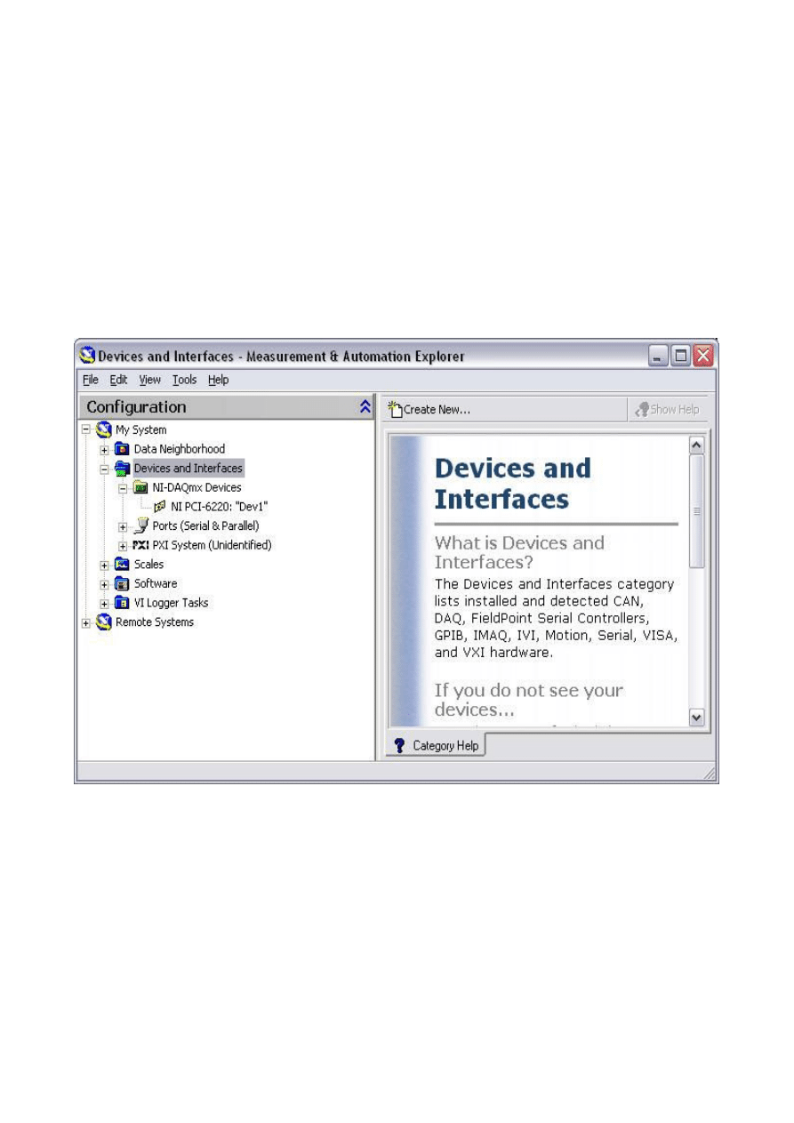
2. Expand the Devices and Interfaces section to view the installed National
Instruments devices. MAX displays the National Instruments hardware and software
in the computer. The device number appears in quotes following the device name.
The data acquisition VIs use this device number to determine which device performs
DAQ operations.
3. Create a simulated DAQ device for use later in this course. Simulated devices are a
powerful tool for development without having hardware physically installed in your
computer. Right-click Devices and Interfaces and select Create New…»NI-
DAQmx Simulated Device. Click “Finish”.
4. Expand the M Series DAQ section. Select PCI-6220 or any other PCI device of your
choice. Click “OK”.
5. The NI-DAQmx Devices folder will expand and you will see a new entry for PCI-
6220: “Dev1”. You have now created a simulated device!
6. Perform a self-test on the device by right-clicking it in the configuration tree and
choosing Self-Test or clicking “Self-Test” along the top of the window. This tests the
system resources assigned to the device. The device should pass the test because it is
already configured.
7. Check the pinout for your device. Right-click the device in the configuration tree and
select Device Pinouts or click “Device Pinouts” along the top of the center window.
8. Open the test panels. Right-click the device in the configuration tree and select Test
Panels… or click “Test Panels…” along the top of the center window. The test
panels allow you to test the available functionality of your device, analog
input/output, digital input/output, and counter input/output without doing any
programming.
9. On the Analog Input tab of the test panels, change Mode to “Continuous”. Click
“Start” and observe the signal that is plotted. Click “Stop” when you are done.
10. On the Digital I/O tab notice that initially the port is configured to be all input.
Observe under Select State the LEDs that represent the state of the input lines. Click
the “All Output” button under Select Direction. Notice you now have switches under
Select State to specify the output state of the different lines. Click “Close” to close
the test panels.
11. Close MAX.
(End of Exercise)
Exercise 1.1 – Setting Up Your Device (Track C)
In this exercise, you will use Windows utilities to verify your sound card and prepare it
for use with a microphone.
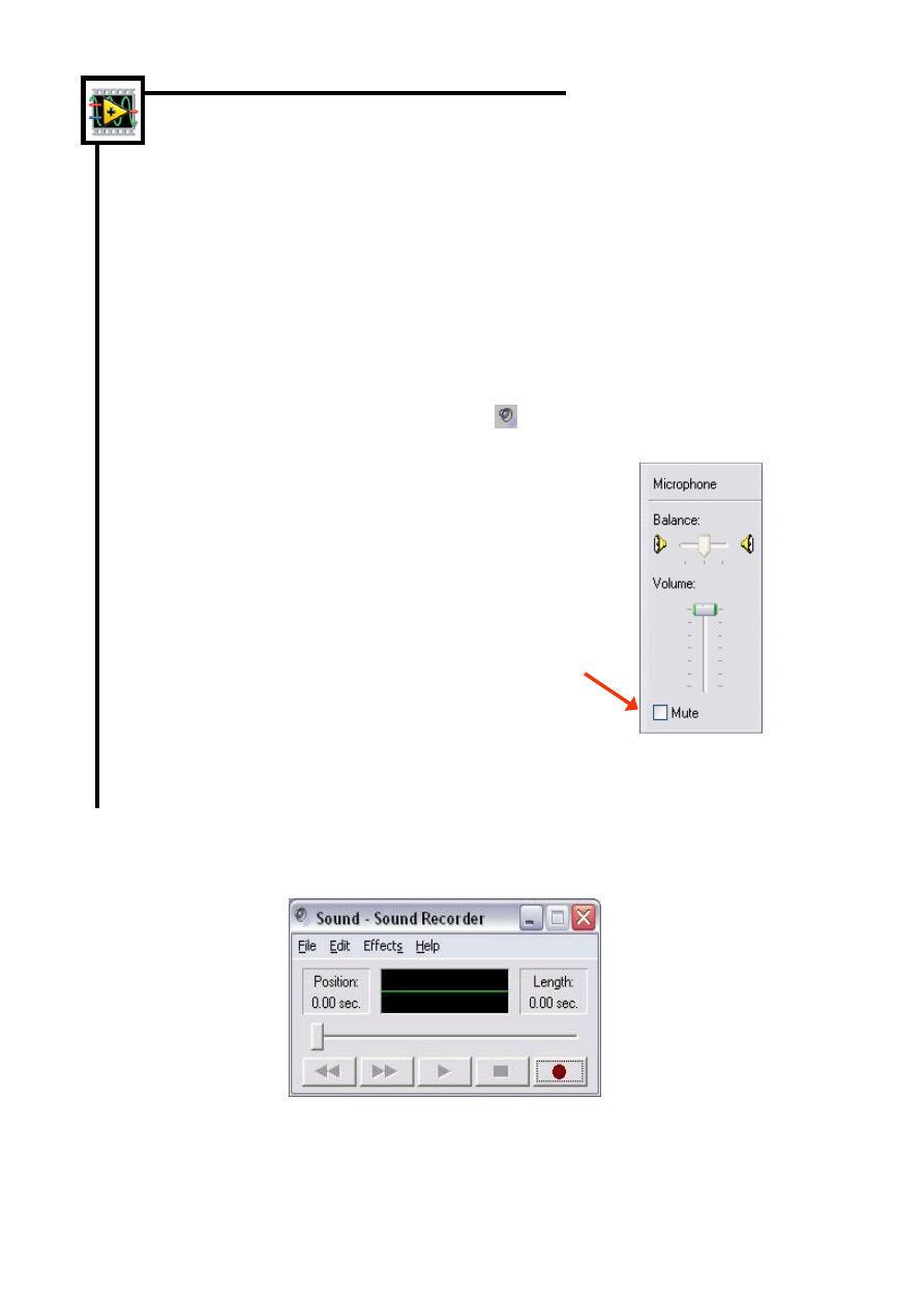
1. Prepare your microphone for use. Double-click the volume control icon on the task
bar to open up the configuration window. The sound configuration window can also
be found from the Windows Control Panel: Start Menu»Control Panel»Sounds
and Audio Devices»Advanced.
2. If you do not see a microphone section, go to Options»Properties»Recording and
place a checkmark in the box next to Microphone. This will display the Microphone
volume control. Click “OK”.
3. Uncheck the Mute box if it is not already unchecked. Make sure that the volume is
turned up.
4. Close the volume control configuration window.
5. Open the Sound Recorder by selecting
Start»Programs»Accessories»Entertainment»Sound Recorder.
6. Click the record button and speak into your microphone. Notice how the sound signal
is displayed in the Sound Recorder.
7. Click stop and close the Sound Recorder without saving changes when you are
finished.
Uncheck Mute
(End of Exercise)

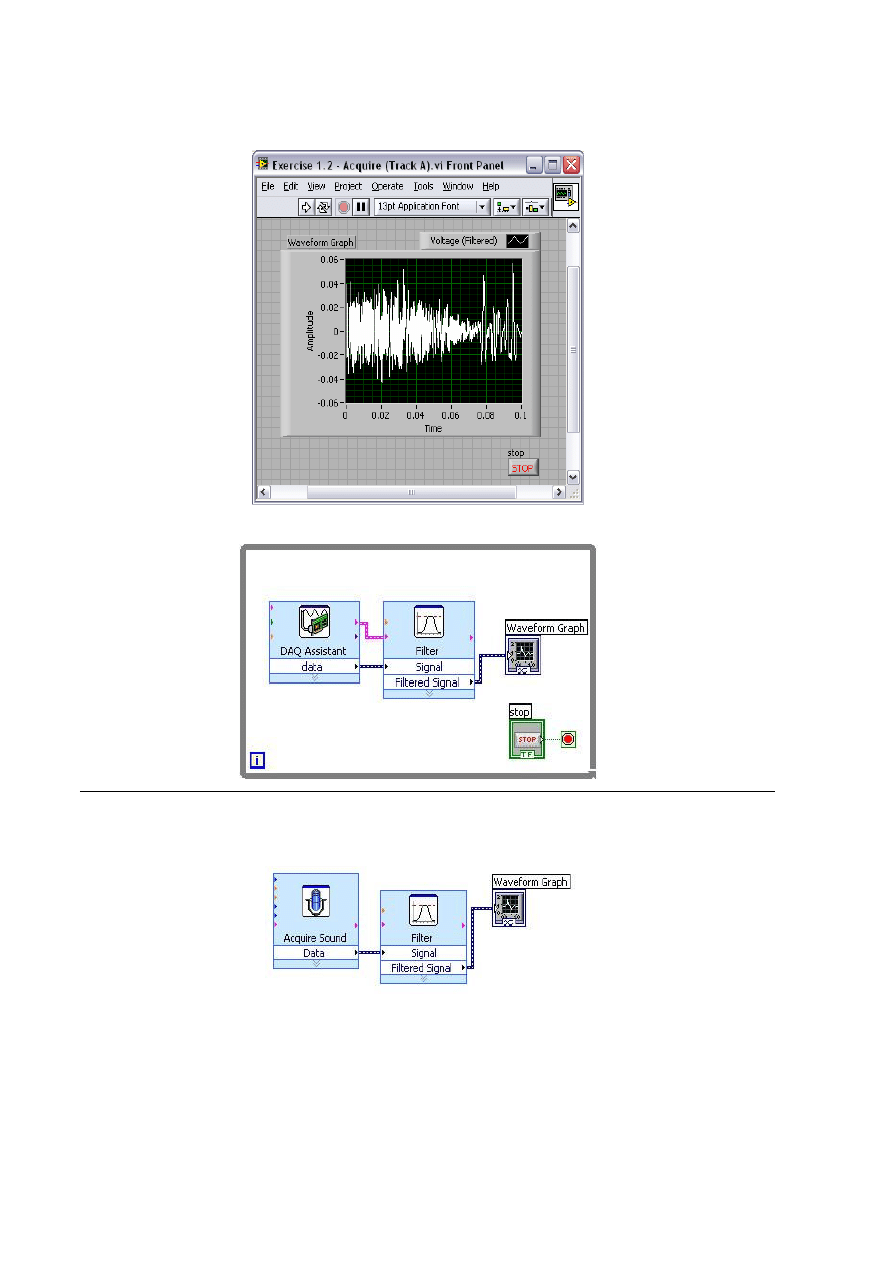
Exercise 1.2 – Acquiring a Signal with DAQ (Track A)
Note: Before beginning this exercise, copy the Exercises and Solutions Folders to the
desktop of your computer.
Complete the following steps to create a VI that acquires data continuously from your
DAQ device.
1. Launch LabVIEW.
2. In the Getting Started window, click the New or VI from Template link to display
the New dialog box.
3. Open a data acquisition template. From the Create New list, select VI»From
Template»DAQ»Data Acquisition with NI-DAQmx.vi and click “OK”.
4. Display the block diagram by clicking it or by selecting Window»Show Block
Diagram. Read the instructions written there about how to complete the program.
5. Double-click the DAQ Assistant to launch the configuration wizard.
6. Configure an analog input operation.
a. Choose Analog Input»Voltage.
b. Choose Dev1 (USB-6009)»ai0 to acquire data on analog input channel 0 and
click “Finish.”
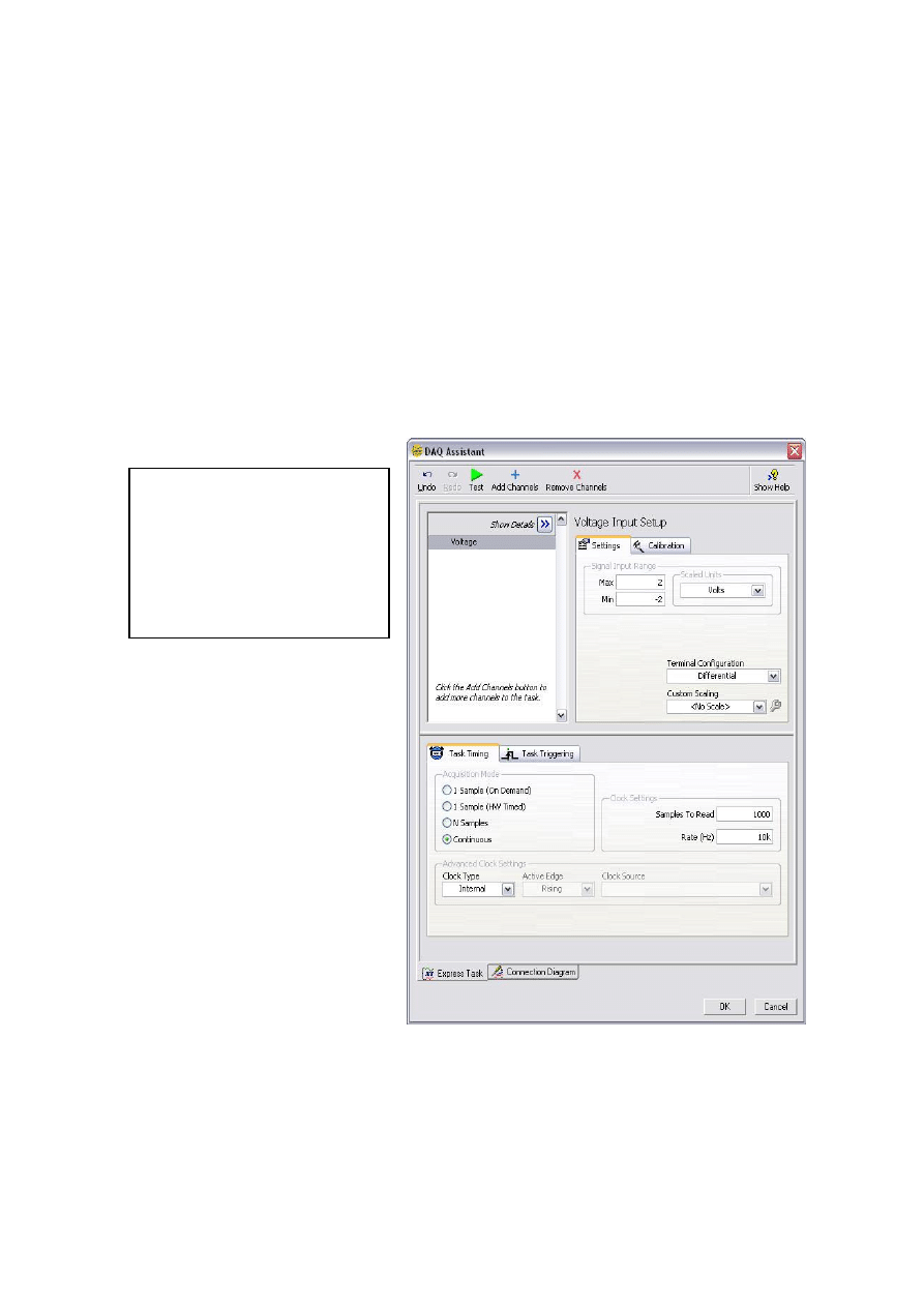
c. In the next window you define parameters of your analog input operation.
To choose an input range that works well with your microphone, on the settings
tab enter 2 Volts for the maximum and –2 Volts for the minimum. On the task
timing tab, choose “Continuous” for the acquisition mode and enter 10000 for
the rate. Leave all other choices set to their default values. Click “OK” to exit
the wizard.
7. Place the Filter Express VI to the right of the DAQ Assistant on the block diagram.
From the functions palette, select Express»Signal Analysis»Filter and place it on the
block diagram inside the while loop. When you bring up the functions palette, press
the small push pin in the upper left hand corner of the palette. This will tack down the
palette so that it doesn’t disappear. This step will be omitted in the following
exercises, but should be repeated. In the configuration window under Filtering Type,
choose “Highpass.” Under Cutoff Frequency, use a value of 300 Hz. Click “OK.”
8. Make the following connections on the block diagram by hovering your mouse over the
terminal so that it becomes the wiring tool and clicking once on each of the terminals you
wish to connect:
a. Connect the “Data” output terminal of the DAQ Assistant VI to the “Signal” input of
the Filter VI.
b. Create a graph indicator for the filtered signal by right-clicking on the “Filtered Signal”
output
terminal and choose Create»Graph Indicator.
9. Return to the front panel by selecting Window»Show Front Panel or by pressing
<Ctrl+E>.
10. Run your program by clicking the run button. Hum or whistle into the microphone to
observe the changing voltage on the graph.
11. Click stop once you are finished.
12. Save the VI as “Exercise 2 – Acquire.vi” in your Exercises folder and close it.
Note: The solution to this exercise is printed in the back of this manual.
Tip: You can place the DAQ
Assistant on your block
diagram from the Functions
Palette. Right-click the block
diagram to open the Functions
Palette and go to
Express»Input to find it.
(End of Exercise)

Exercise 1.2 – Acquiring a Signal with DAQ (Track B)
Note: Before beginning this exercise, copy the Exercises and Solutions Folders to the
desktop
of your computer.
Complete the following steps to create a VI that acquires data continuously from your
simulated DAQ device.
1. Launch LabVIEW.
2. In the Getting Started window, click the New or VI from Template link to display the
New dialog box.
3. Open a data acquisition template. From the Create New list, select VI»From
Template»DAQ»Data Acquisition with NI-DAQmx.vi and click “OK”.
4. Display the block diagram by clicking it or by selecting Window»Show Block Diagram.
Read the instructions written there about how to complete the program.
5. Double-click the DAQ Assistant to launch the configuration wizard.
6. Configure an analog input operation.
a. Choose Analog Input»Voltage.
b. Choose Dev1 (PCI-6220)»ai0 to acquire data on analog input channel 0
and click “Finish.”
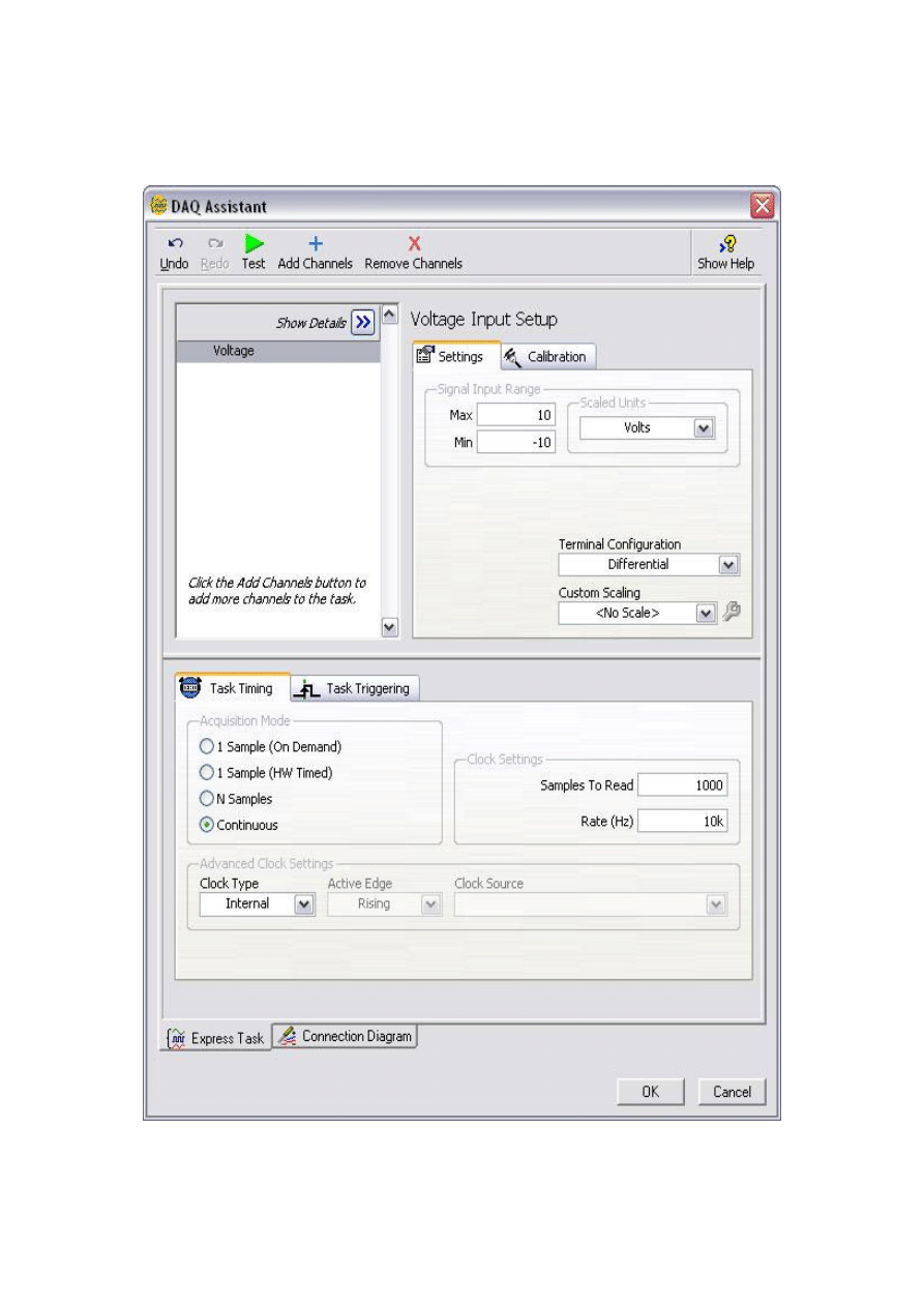
c. In the next window you define parameters of your analog input operation.
On the task timing tab, choose “Continuous” for the acquisition mode,
enter 1000 for samples to read, and 10000 for the rate. Leave all other
choices set to their default values. Click “OK” to exit the wizard.
7. On the block diagram, right-click the black arrow to the right of where it says “data.”
Choose Create»Graph Indicator from the right-click menu.
8. Return to the front panel by selecting Window»Show Front Panel or by pressing
<Ctrl+E>.
9. Run your program by clicking the run button. Observe the simulated sine wave on the
graph.
10. Click stop once you are finished.
11. Save the VI as “Exercise 2 – Acquire.vi” in the Exercises folder. Close the VI.
Notes:
•
The solution to this exercise is printed in the back of this manual.
•
You can place the DAQ Assistant on your block diagram from the Functions Palette.
Right-click the block diagram to open the Functions Palette and go to Express»Input
to find it. When you bring up the functions palette, press the small push pin in the upper
left hand corner of the palette. This will tack down the palette so that it doesn’t
disappear. This step will be omitted in the following exercises, but should be repeated.
(End of Exercise)

Exercise 1.2 – Acquiring a Signal with the Sound Card (Track C)
Note: Before beginning this exercise, copy the Exercises and Solutions Folders to
the desktop of your computer.
Complete the following steps to create a VI that acquires data from your sound card.
1. Launch LabVIEW.
2. In the Getting Started window, click the Blank VI link.
3. Display the block diagram by pressing <Ctrl+E> or selecting Window»Show Block
Diagram.
4. Place the Acquire Sound Express VI on the block diagram. Right-click to open the
functions palette and select Express»Input»Acquire Sound. Place the Express VI
on the block diagram.
5. In the configuration window under #Channels, select 1 from the drop-down list and
click “OK”.
6. Place the Filter Express VI to the right of the Acquire Signal VI on the block
diagram. From the functions palette, select Express»Signal Analysis»Filter and
place it on the block diagram. In the configuration window under Filtering Type,
choose “Highpass.” Under Cutoff Frequency, use a value of 300 Hz. Click “OK.”
7. Make the following connections on the block diagram by hovering your mouse over
the terminal so that it becomes the wiring tool and clicking once on each of the
terminals you wish to connect:
a. Connect the “Data” output terminal of the Acquire Signal VI to the “Signal” input
of the Filter VI.
b. Create a graph indicator for the filtered signal by right-clicking on the “Filtered
Signal” output terminal and choose Create»Graph Indicator.
8. Return to the front panel by pressing <Ctrl+E> or Window»Show Front Panel.
9. Run your program by clicking the run button. Hum or whistle into your microphone
and observe the data you acquire from your sound card.
10. Save the VI as “Exercise 1.2 – Acquire.vi” in the Exercises folder.
11. Close the VI.
Note: The solution to this exercise is printed in the back of this manual.
(End of Exercise)
Exercise 2.1 – Analysis (Track A, B, & C)
Create a VI that produces a sine wave with a specified frequency and displays the data
on a Waveform Chart until stopped by the user.
1. Open a blank VI from the Getting Started screen.
2. Place a chart on the front panel. Right-click to open the controls palette and select
Controls»Modern»Graph»Waveform Chart.
3. Place a dial control on the front panel. From the controls palette, select
Controls»Modern »Numeric»Dial. Notice that when you first place the control on
the front panel, the label text is highlighted. While this text is highlighted, type
“Frequency In” to give a name to this control.
4. Go to the block diagram (<Ctrl+E>) and place a while loop down. Right-click to
open the functions palette and select Express»Execution Control»While Loop.
Click and drag on the block diagram to make the while loop the correct size. Select
the waveform chart and dial and drag them inside the while loop if they are not
already. Notice that a stop button is already connected to the conditional terminal of
the while loop.
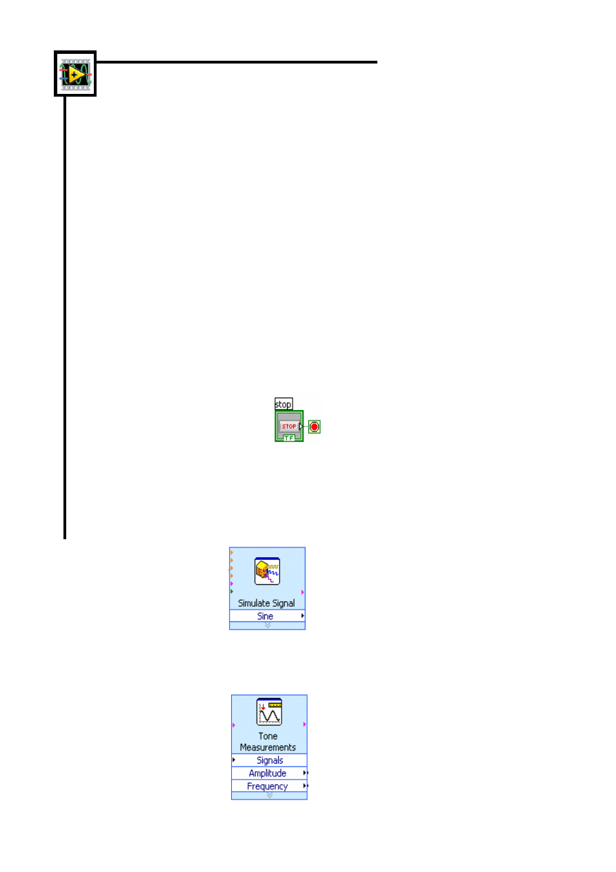
5. Place the Simulate Signal Express VI on the block diagram. From the functions
palette, select Express»Signal Analysis»Simulate Signal and place it on the block
diagram inside the while loop. In the configuration window under Timing, choose
“Simulate acquisition timing.” Click “OK.”
6. Place a Tone Measurements Express VI on the block diagram (Express»Signal
Analysis»Tone Measurements). In the configuration window, choose Amplitude
and Frequency measurements in the Single Tone Measurements section. Click “OK.”

7. Make the following connections on the block diagram by hovering your mouse over
the terminal so that it becomes the wiring tool and clicking once on each of the
terminals you wish to connect:
a. Connect the “Sine” output terminal of the Simulate Signal VI to the
“Signals” input of the Tone Measurements VI.
b. Connect the “Sine” output to the Waveform Chart.
c. Create indicators for the amplitude and frequency measurements by right-clicking
on each of the terminals of the Tone Measurements Express VI and selecting
Create»Numeric Indicator.
d. Connect the “Frequency In” control to the “Frequency” terminal of the
Simulate Signal VI.
8. Return to the front panel and run the VI. Move the “Frequency In” dial and observe
the frequency of the signal. Click the stop button once you are finished.
9. Save the VI as “Exercise 2.1 – Simulated.vi”.
10. Close the VI.
Notes
•
When you bring up the functions palette, press the small push pin in the upper left
hand corner of the palette. This will tack down the palette so that it doesn’t disappear.
This step will be omitted in the following exercises, but should be repeated.
•
The solution to this exercise is printed in the back of this manual.
(End of Exercise)

Exercise 2.2 – Analysis (Track A & B)
Create a VI that measures the frequency and amplitude of the signal from your
(simulated) DAQ device and displays the acquired signal on a waveform chart. The
instructions are the same as in Exercise 2.1, but a DAQ Assistant is used in place of the
Simulate Signal VI. Try to do this without following the instructions!
1. Open a blank VI.
2. Place a chart on the front panel. Right click to open the controls palette and select
Controls»Modern»Graph»Waveform Chart.
3. Go to the block diagram and place a while loop down (Express»Execution
Control»While Loop).
4. Place a DAQ Assistant on the block diagram (Express»Input»DAQ Assistant).
Choose analog input on channel ai0 of your (simulated) device and click “Finish.”
On the task timing tab, choose “continuous” for the acquisition mode. If you are
using the USB-6009, change the Input Range to -2 to 2 and the number of Samples
to Read to 100.
5. Place the Filter Express VI to the right of the DAQ Assistant on the block diagram.
From the functions palette, select Express»Signal Analysis»Filter and place it on
the block diagram inside the while loop. In the configuration window under Filtering
Type, choose “Highpass.” Under Cutoff Frequency, use a value of 300 Hz. Click
“OK.”
6. Connect the “Data” output terminal of the DAQ Assistant VI to the “Signal” input of
the Filter VI.
7. Connect the “Filtered Signal” terminal on the Filter VI to the Waveform Chart.
8. Place a Tone Measurements Express VI on the block diagram (Express»Signal
Analysis»Tone). In the configuration window, choose Amplitude and Frequency
measurements in the Single Tone Measurements section.
9. Create indicators for the amplitude and frequency measurements by right clicking on
each of the terminals of the Tone Measurements Express VI and selecting
Create»Numeric Indicator.
10. Connect the output of the Filter VI to the “Signals” input of the Tone Measurements
Express VI.
11. Return to the front panel and run the VI. Observe your acquired signal and its
frequency and amplitude. Hum or whistle into the microphone if you have a USB-
6009 and observe the amplitude and frequency that you are producing.
12. Save the VI as “Exercise 2.2 - Data.vi”.
13. Close the VI.
Note: The solution to this exercise is printed in the back of this manual.
(End of Exercise)

Exercise 2.2 – Analysis (Track C)
Create a VI that measures the frequency and amplitude of the signal from your sound card
and displays the acquired signal on a waveform chart. The instructions are the same
as in Exercise 2.1, but the Sound Signal VI is used in place of the Simulate Signal VI.
Try to do this without following the instructions!
1. Open a blank VI.
2. Go to the block diagram and place a While Loop down (Express»Execution
Control»While Loop).
3. Place the Acquire Sound Express VI on the block diagram (Express»Input»
Acquire Sound).
4. Place a Filter Express VI on the block diagram. In the configuration window choose a
highpass filter and a cutoff frequency of 300 Hz.
5. Place a Tone Measurements Express VI on the block diagram (Express»Signal
Analysis»Tone). In the configuration window, choose Amplitude and Frequency
measurements in the Single Tone Measurements section.
6. Create indicators for the amplitude and frequency measurements by right-clicking on
each of the terminals of the Tone Measurements Express VI and selecting
Create»Numeric Indicator.
7. Connect the “Data” terminal of the Acquire Sound Express VI to the “Signal” input
of the Filter VI.
8. Connect the “Filtered Signal” terminal of the Filter VI to the “Signals” input of the
Tone Measurements VI.
9. Create a graph indicator for the Filtered Signal by right-clicking on the “Filtered
Signal” terminal and selecting Create»Graph Indicator.
10. Return to the front panel and run the VI. Observe the signal from your sound card
and its amplitude and frequency. Hum or whistle into the microphone and observe the
amplitude and frequency you are producing.
11. Save the VI as “Exercise 2.2-Data.vi”. Close the VI.
Note: The solution to this exercise is printed in the back of this manual.
(End of Exercise)
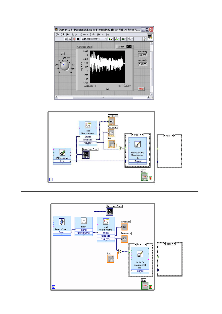
Exercise 2.3 – Decision Making and Saving Data (Track A, B, & C)
Create a VI that allows you to save your data to file if the frequency of your data
goes below a user-controlled limit.
1. Open Exercise 3.2 – Data.vi.
2. Go to File»Save As… and save it as “Exercise 3.3 – Decision Making and Saving
Data”. In the “Save As” dialog box, make sure substitute copy for original is
selected and click “Continue…”.
3. Add a case structure to the block diagram inside the while loop
(Functions»Programming»Structures»Case Structure).
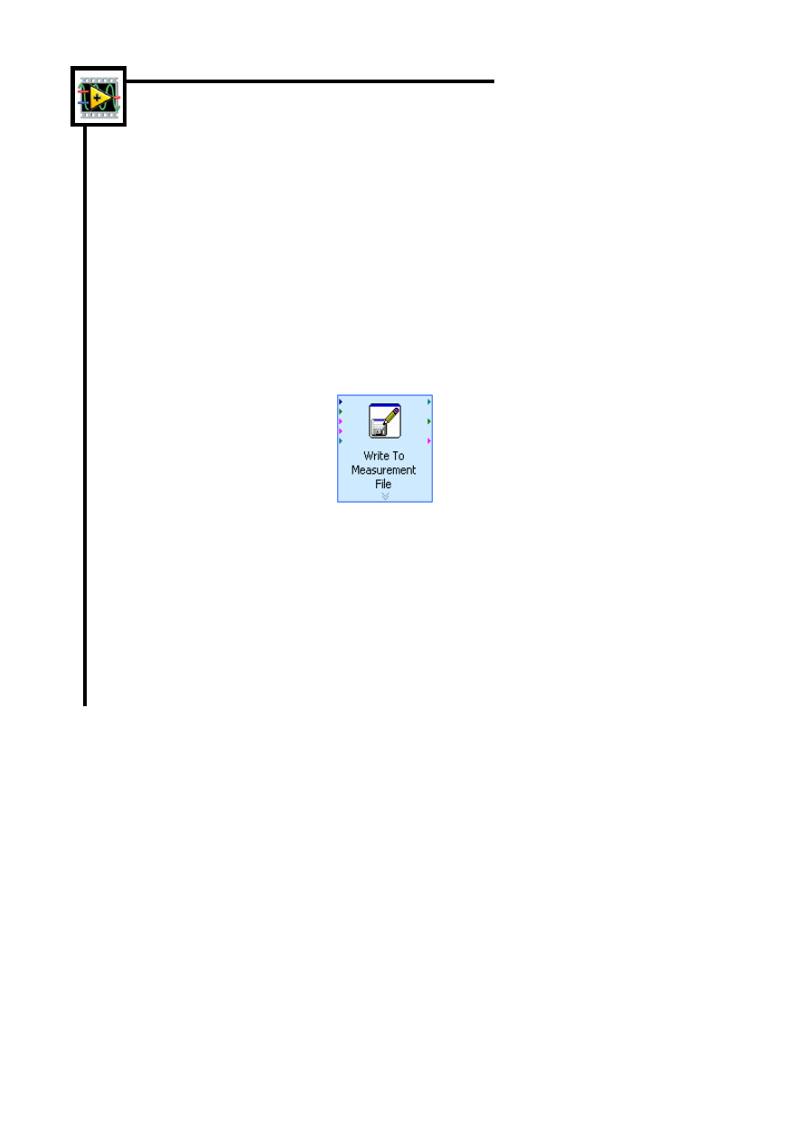
4. Inside the “true” case of the case structure, add a Write to Measurement File Express
VI (Functions»Programming»File I/O»Write to Measurement File).
a. In the configuration window that opens, choose “Save to series of files
(multiple files).” Note the default location your file will be saved to and change
it if you wish.
b. Click “Settings…” and choose “Use next available file name” under the
Existing Files heading.
c. Under File Termination choose to start a new file after 10 segments. Click
“OK” twice.
5. Add code so that if the frequency computed from the Tone Measurements Express VI
goes below a user-controlled limit, the data will be saved to file. Hint: Go to
Functions»Programming»Comparison»Less?
6. Remember to connect your data from the DAQ Assistant or Acquire Sound Express
VI to the “Signals” input of the Write to Measurement File VI. If you need help, refer
to the solution to this exercise.
7. Go to the front panel and run your VI. Vary your frequency limit and then stop the
VI.
8. Navigate to My Documents»LabVIEW Data and open one of the files that was
saved there. Examine the file structure and check to verify that 10 segments are in the
file.
9. Save your VI and close it.
Note: The solution to this exercise is printed in the back of this manual.
(End of Exercise)

Exercise 2.4 – Write to Spreadsheet File
1.
Open a blank new VI from the Getting Started screen.
2.
Place the Open/Create/Replace File function on the block diagram. Right-click on the block
diagram to open the functions palette and select File I/O » Open/Create/Replace File.
3.
Right-click the operation terminal of the Open/Create/Replace File function and select Create »
Constant from the shortcut menu, and select open or create from the drop down menu.
4.
Place a While loop from the Structures palette on the block diagram to the right of the
Open/Create/Replace File function. Right-click on the block diagram select Structures » While
Loop.
5.
Place a Write Text File function inside the While Loop. Right-click on the block diagram select
File I/O » Write To Text File.
6.
Wire the refnum out terminal from the Open/Create/Replace File function to the file (use dialog)
terminal of the Write Text File function.
7.
Wire the error out terminal from the Open/Create/Replace File function to the error in terminal
of the Write Text File function.
8.
Place an Array to Spreadsheet String function inside the while loop and to the left of the on
Open/Create/Replace File function. Right-click on the block diagram and select String » Array to
Spreadsheet String.
9.
Right-click the format string terminal of the Array to Spreadsheet function and select Create »
Constant from the shortcut menu and enter “%0.4f” in the string constant to format the input
data.
10. Place a Build Array Function on the block diagram. Right-click on the block diagram and select
Array » Build Array.
11. Place a Random Number inside the While Loop. Right-click on the block diagram and select
Numeric » Random Number (0-1).
12. Wire the error out terminal of the Write Text File function to an output tunnel on the While
Loop.
13. Place an Unbundle By Name function inside the While Loop. Right-click on the block diagram to
open the functions palette and select Cluster & Variant » Unbundle By Name.
14. Wire the error out from the Write Text File function to the Unbundle By Name function.
15. Place an Or function in the While Loop. Right-click on the block diagram to open the
functions palette and select Boolean » Or.
16. Switch to the front panel and place a stop button. Right-Click on the front panel to open
the Controls palette and select Boolean » Stop Button.
17. On the block diagram, wire the status element of the error cluster to the x input of the
Or function and wire the stop button to the y input.
18. Wire the output of the Or function to the conditional terminal of the While Loop.
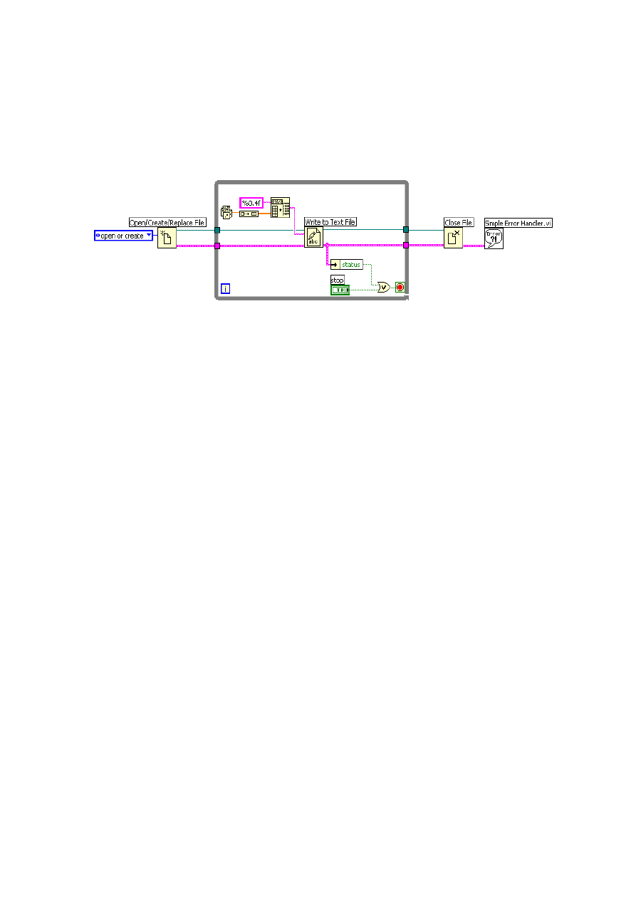
19. Place a Close File function to the right of the While Loop. Right-click on the block diagram to
open the functions palette and select File I/O » Close File.
20. Wire the refnum output tunnel to the refnum input terminal of the Close File function.
21. Wire the error output tunnel to the error in terminal of the Close File function.
22. Return to the front panel and run the VI. You will be prompted to “Choose or enter path of file
to open”, enter: “spreadsheet.xls”.
23. Click on the stop button to stop the execution of the VI.
24. Open the file named: “spreadsheet.xls”.
25. Save and the close the VI.
(End of Exercise)
Exercise 3.1 – Manual Analysis (Track A, B, & C)
Create a VI that displays simulated data on a waveform graph and measures the
frequency and amplitude of that data. Use cursors on the graph to verify the
frequency and amplitude measurements.
1. Open Exercise 2.1 – Simulated.vi.
2. Save the VI as “Exercise 3.1 – Manual Analysis.vi”.
3. Go to the block diagram and remove the While Loop. Right-click the edge of the loop
and choose Remove While Loop so that the code inside the loop does not get
deleted.
4. Delete the stop button.
5. On the front panel, replace the waveform chart with a waveform graph. Right-click
the chart and select Replace»Modern»Graph»Waveform Graph.
6. Make the cursor legend viewable on the graph. Right-click on the graph and select
Visible Items»Cursor Legend.
7. Change the maximum value of the “Frequency In” dial to 100. Double-click on the
maximum value and type “100” once the text is highlighted.
8. Set a default value for the “Frequency In” dial by setting the dial to the value you
would like, right-clicking the dial, and selecting Data Operations»Make Current
Value Default.
9. Run the VI and observe the signal on the waveform graph. If you cannot see the
signal, you may need to turn on auto-scaling for the x-axis. Right-click on the graph
and select X Scale»AutoScale X.
10. Change the frequency of the signal so you can see a few periods on the graph.
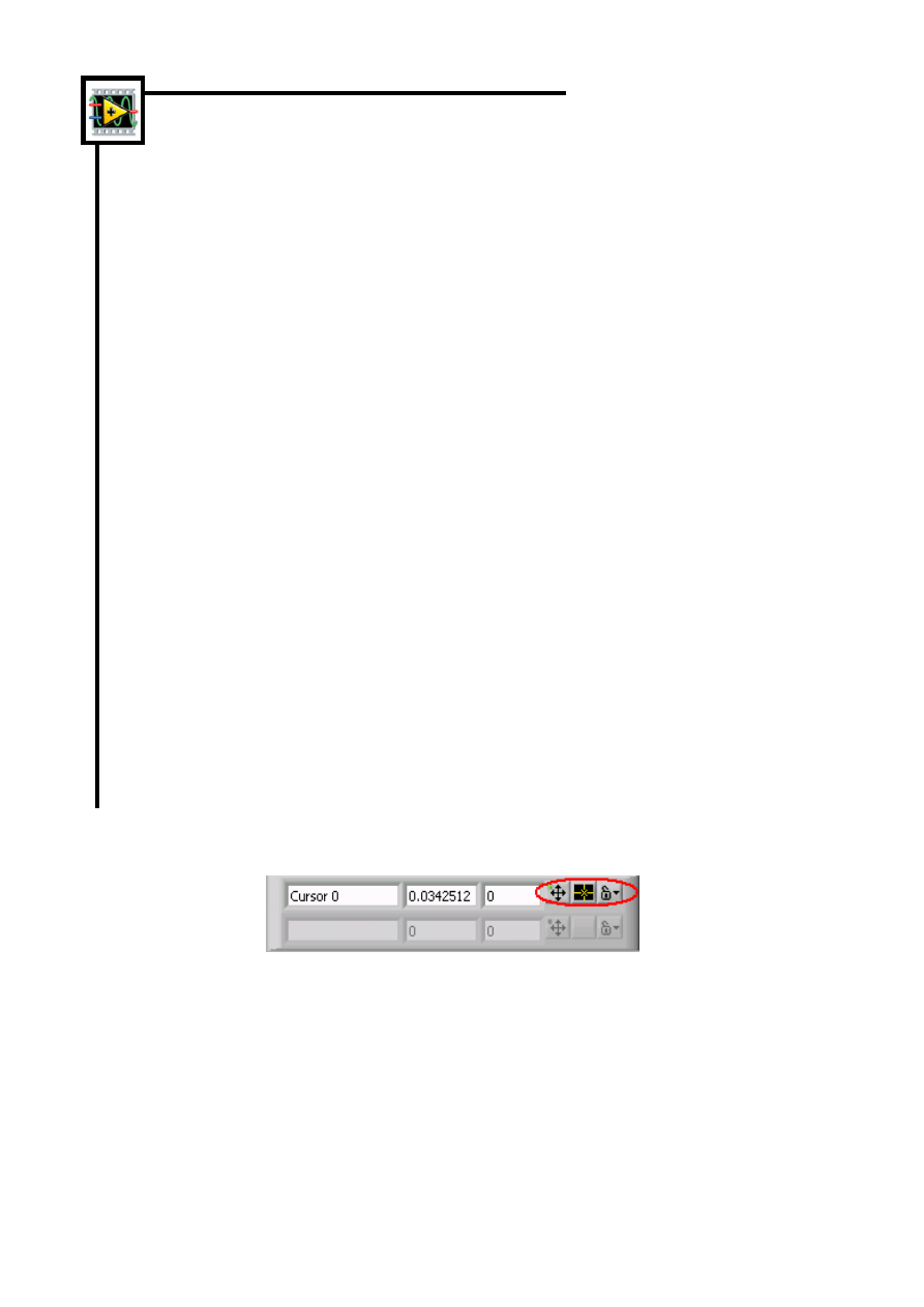
11. Manually measure the frequency and amplitude of the signal on the graph using
cursors. To make the cursors display on the graph, click on one of the three buttons in
the cursor legend. Once the cursors are displayed, you can drag them around on the
graph and their coordinates will be displayed in the cursor legend.
12. Remember that the frequency of a signal is the reciprocal of its period (f = 1/T). Does
your measurement match the frequency and amplitude indicators from the Tone
Measurements VI?
13. Save your VI and close it.
Note: The solution to this exercise is printed in the back of this manual.
(End of Exercise)

Exercise 3.2 – MathScript (Track A, B, & C)
Create a VI that uses the MathScript Node to alter your simulated signal and graph it. Use
the Interactive MathScript Window to view and alter the data and then load the script you
have created back into the MathScript Node.
1. Open Exercise 3.1 – Manual Analysis.vi.
2. Save the VI as “Exercise 3.2 – MathScript.vi”.
3. Go to the block diagram and delete the wire connecting the Simulate Signal VI to the
Waveform Graph.
4. Place down a MathScript Node (Programming»Structures»MathScript Node).
5. Right-click on the left border of the MathScript Node and select Add Input. Name
this input “In” by typing while the input node is highlighted black.
6. Right-click on the right border of the MathScript Node and select Add Output.
Name this output “Out”.
7. Convert the Dynamic Data Type output of the Simulate Signals VI to a 1D Array of
Scalars to input to the MathScript Node. Place a Convert from Dynamic Data
Express VI on the block diagram (Express»Signal Manipulation»Convert from
Dynamic Data). By default, the VI is configured correctly so click “OK” in the
configuration window.
8. Wire the “Sine” output of the Simulate Signal VI to the “Dynamic Data” input of the
Convert from Dynamic Data VI.
9. Wire the “Array” output of the Convert from Dynamic Data VI to the “In” node on
the MathScript Node.
10. In order to use the data from the Simulate Signal VI in the Interactive MathScript
Window it is necessary to declare the input variable as a global variable. Inside the
MathScript Node type “global In;”.
11. Return to the front panel and increase the frequency to be between 50 and 100. Run
the VI.
12. Open the Interactive MathScript Window (Tools»MathScript Window…).
13. In the MathScript Window, the Command Window can be used to enter in the
command that you wish to compute. In the Command Window, type “global In” and
press “Enter”. This will allow you to see the data passed to the variable “In” on the
MathScript Node.
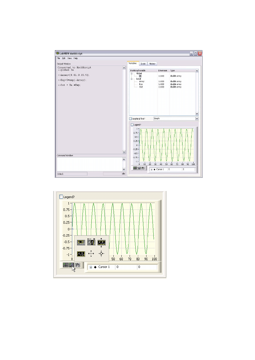
14. Notice that all declared variables in the script along with their dimensions and type are listed
on the “Variables” tab. To display the graphed data, click once on the variable In and change
the drop down menu from “Numeric” to “Graph”.
15. Use the graph palette to zoom in on your data.
16. Right-click on “Cursor 1” and choose Bring to Center. What does this do?
17. Drag the cursor around. The cursor will not move if the zoom option is selected.
18. Right-click on the graph and choose Undock Window. What does this do? Close this new
window when you are finished.
19. Multiply the data by a decreasing exponential function. Follow these steps:
a. Make a 100 element array of data that constitutes a ramp function going
from 0.01 to 5 by typing “Array = [0.01:0.05:5];” in the Command
Window and pressing Enter. What type of variable is “Array”?
b. Make an array containing a decreasing exponential. Type
“Exp = 5*exp(-Array);” and press Enter.
c. Now multiply the Exp and In arrays element by element by typing
“Out = In.*Exp;” and pressing Enter.
d. Look at the graph of the variable “Out”.
20. Go to the History tab and use Ctrl-click to choose the 4 commands you just entered.
Copy those commands using <Ctrl-C>.
21. On the Script tab, paste the commands into the Script Editor using <Ctrl-V>.
22. Save your script by clicking “Save” at the bottom of the window. Save it as
“myscript.txt”
23. Close the MathScript Window.
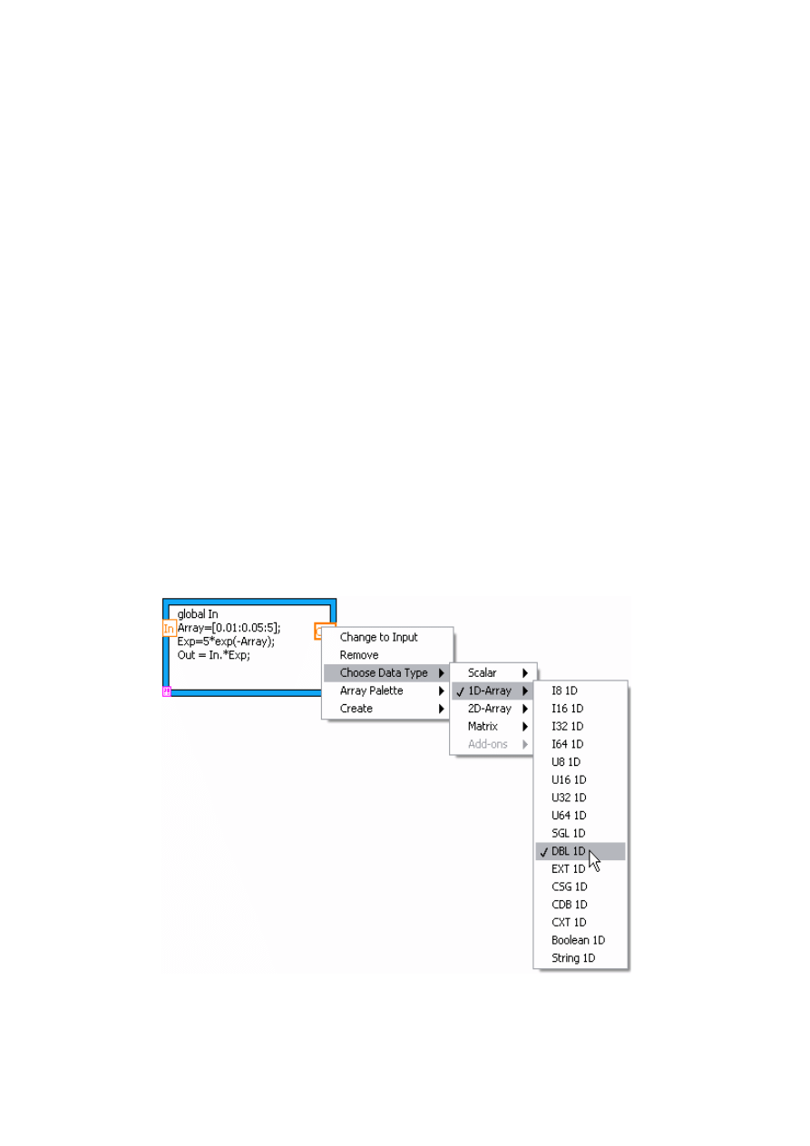
24. Return to the block diagram of Exercise 4.2 – MathScript. Load the script you just made
by right-clicking on the MathScript Node border and selecting Import… Navigate to
myscript.txt, select it, and click “OK”.
25. Right-click on the variable “Out” and select Choose Data Type»1D-Array»DBL 1D.
Output data types must be set manually on the MathScript Node.
26. Wire “Out” to the Waveform Graph.
27. Return to the front panel and run the VI.
Does the data look like you expect?
25. Save and close your VI.
Note: The solution to this exercise is printed in the
back of this manual.
(End of Exercise)
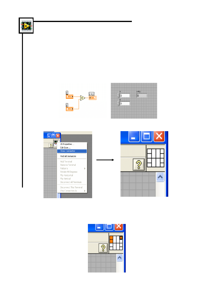
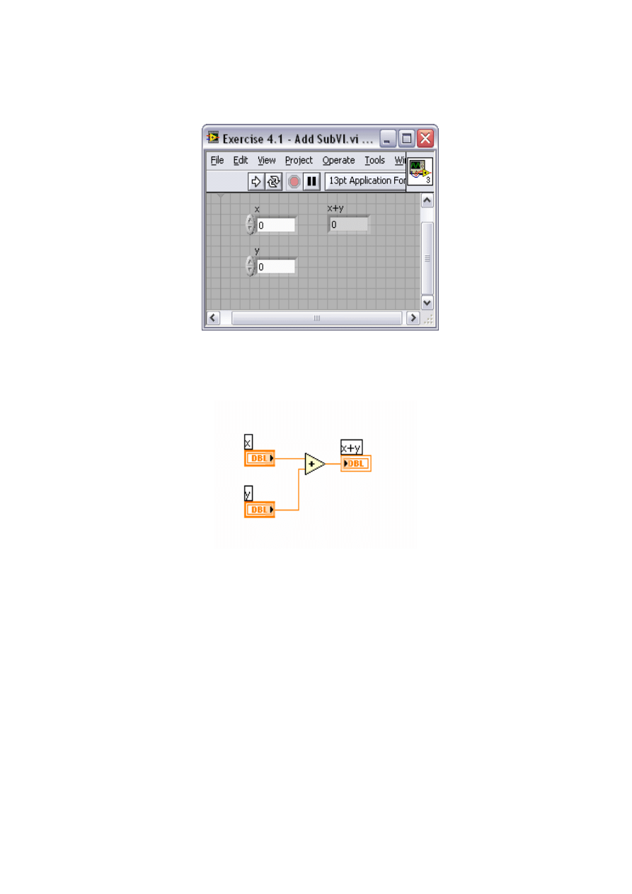
Exercise 4.1 – Creating a SubVI
Create a subVI from a new VI, which adds two inputs and outputs the sum.
1. Open a new VI (Ctrl+N).
2. Place the Add function (Programming » Numeric) on the block diagram.
3. Create controls and indicators by right-clicking and selecting Create » Control or
Indictor. The Block Diagram and Front Panel should look similar to the images
below.
4. On the Front Panel right-click the Icon at the top right and select Show Connector to
reveal the Connector Pane.
5. Assign icon terminals to the two controls and indicators by first left-clicking on a icon
terminal and then clicking the desired control/indicator
Note: General convention is to have controls as data inputs on the left side and
indicators as outputs on the rights side of this icon.
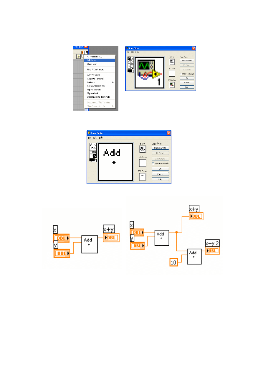
6. Right-click on the Connector Panel and select Edit Icon…. This will bring up the Icon
Editor.
7. Modify the graphics to more accurately represent the function of the SubVI, in this case
Addition.
8. Save the SubVI. It can now be used in any other VI to perform any function, in this case
adding two numbers.
(End of Exercise)
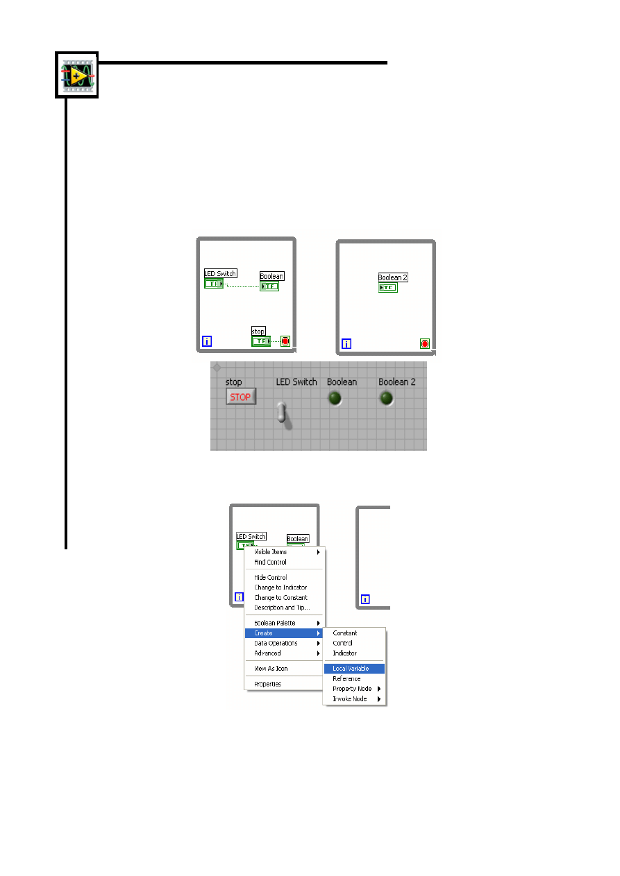
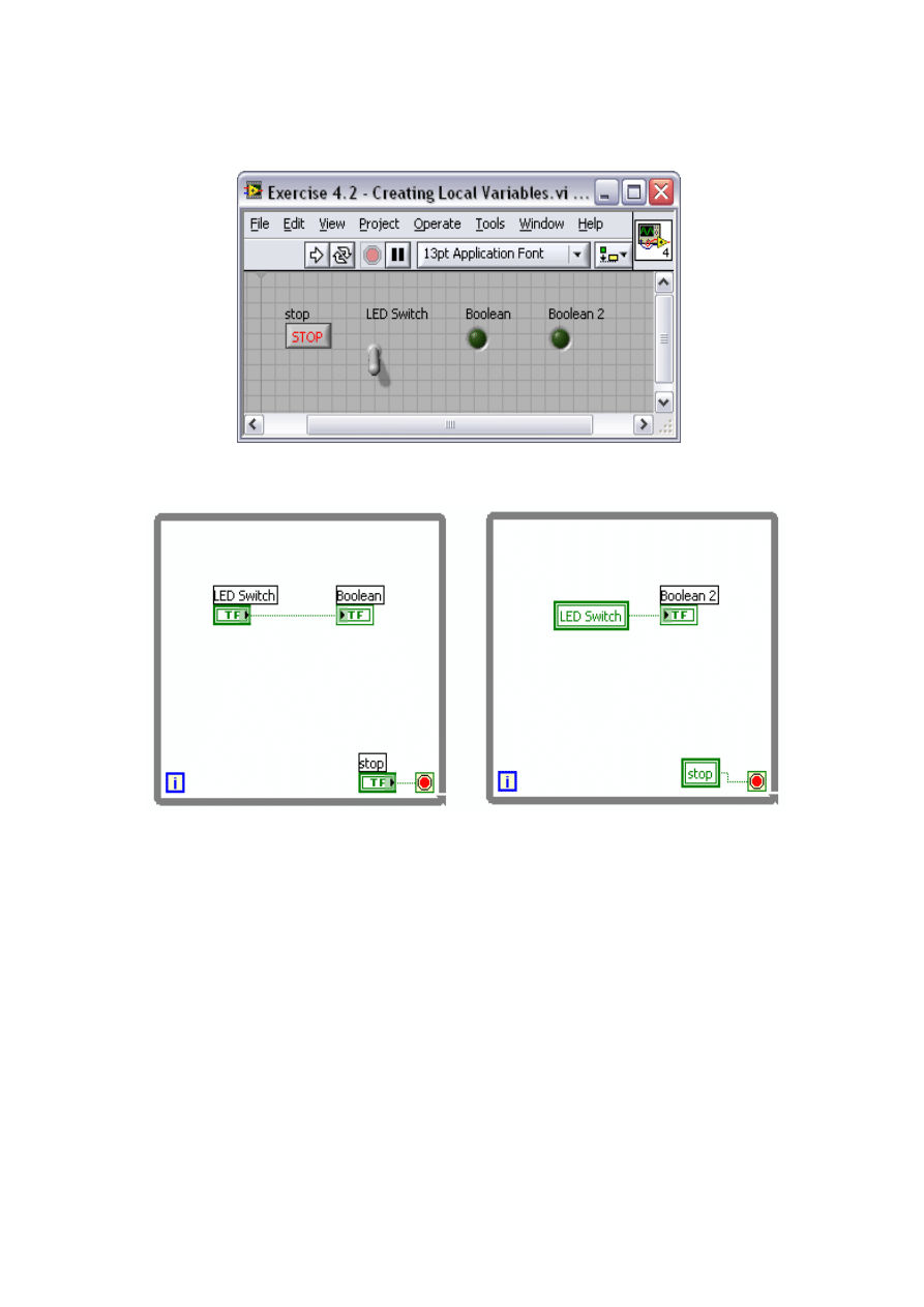
Exercise 4.2 – Creating Local Variables
Create a VI that communicates between two parallel while loops using a Local Variable.
1. Open a new VI.
2. On the Front Panel, place a LED Switch and two Boolean indicators.
3. On the Block Diagram, place two while loops down and create a stop button by right-
clicking on the exit condition terminal and selecting Create » Control.
4. Arrange the code to be similar to the following.
5. Right-click on the LED Switch Control on the Block Diagram and select Create »
Local Variable.
6. Place the new Local Variable in the second while loop.
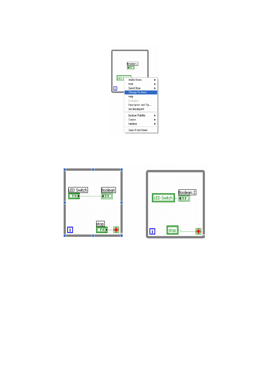
7. Right-click the Variable and select Change To Read. This means that instead of writing data
to local variable we read data already written to the variable.
8. Repeat the process for the Stop button.
9. Right-click on the Stop Button on the Front Panel and change the Mechanical Action to
Switch When Released. Local Variables cannot store latched Boolean data. The finished
code will look as follows:
10. Run the VI. Notice how we can control the LED values and stop two loops with one control.
11. Save the VI.
(End of Exercise)
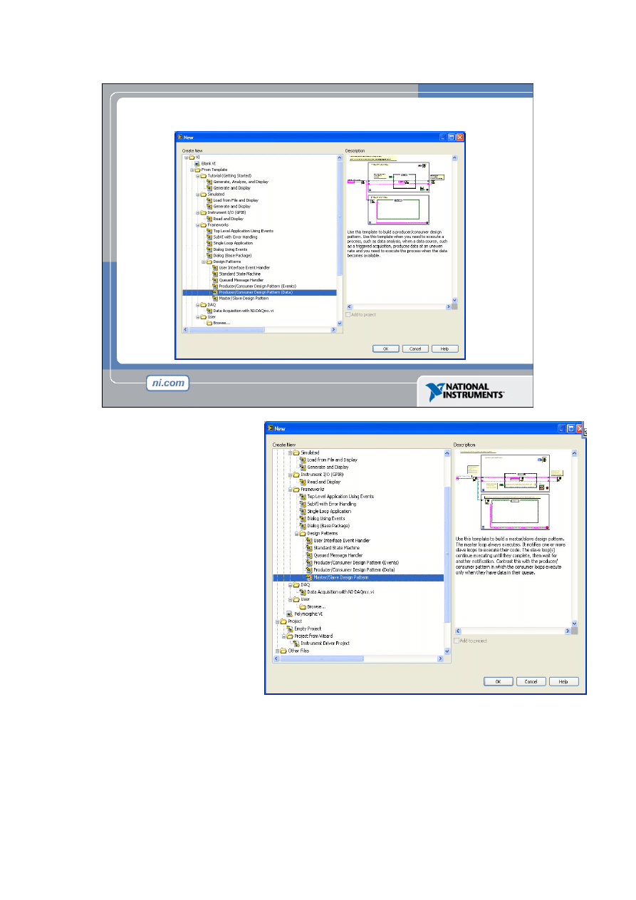
Producer/Consumer Design Pattern
Besides Variables, there are
several other methods for
transferring data between
parallel loops. This is
accomplished using Notifier
and Queue functions. Notifiers
can be used to implement a
Master/Slave design pattern
and Queues are used to
implement a
Producer/Consumer design
pattern. Both enable
LabVIEW programmers to
share data between loops.
Select File » New and navigate
to VI » From Template »
Frameworks » Design
Patterns to see an overview of
both design patterns.
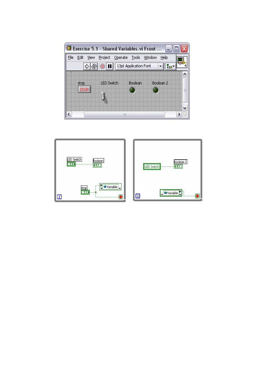
Exercise 5.1 – Shared Variable
Create a Shared Variable from a project and use that Variable instead of the Local Variable
in the exercise created previously.
1. Open the Local Variable VI that was created in Exercise 4.2.
2. Select Project » New Project from the Menu Bar. This will create a new project.
When prompted select Add to add the currently open VI to the project.
3. Save the project by selecting Project » Save Project in the Project Explorer Window.
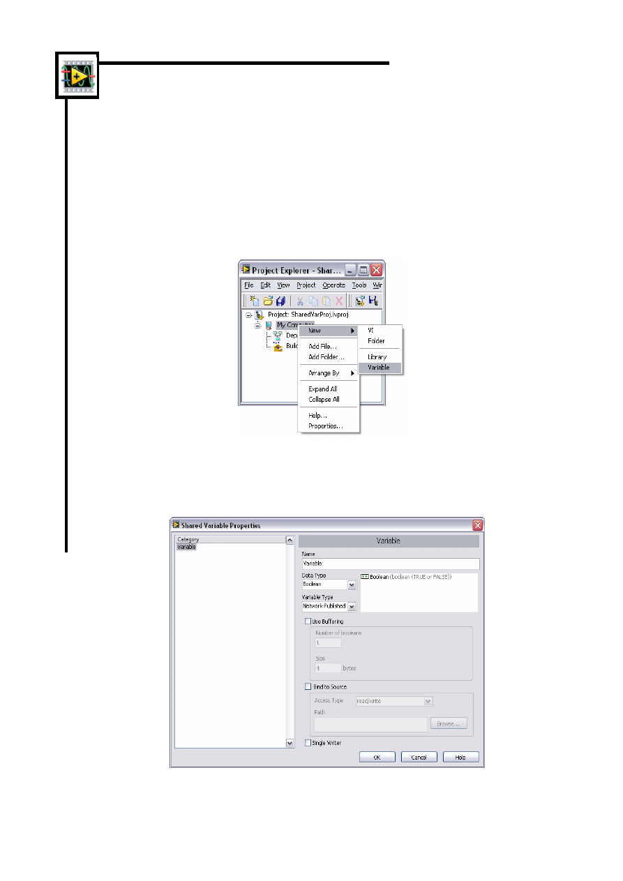
4. Create a Shared Variable by right-clicking on My Computer and selecting New »
Variable.
5. In the configuration window, name the Variable and select Boolean from the Data Type
drop down menu. Leave the rest of the options as default and click OK.
6. Since Shared Variables need a to reside in a Library, LabVIEW creates one. Save
this Library by right-clicking and selecting Save.
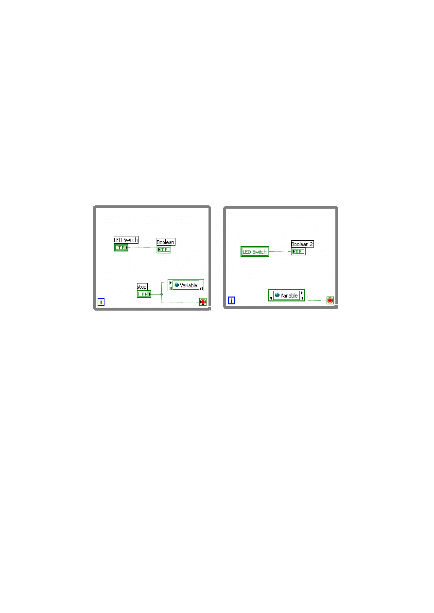
7. Shared Variables can easily be used by clicking and dragging from the Project
Explorer to the VI. Click and drag the Shared Variable you created to the Block
Diagram on the open Local Variable VI.
8. Delete the Local Variable that controls the stop button in the second loop.
9. Place the variable in the second loop and wire the variable to the exit terminal.
10. Place another copy of the Shared Variable in the first loop. This Shared Variable will
write the information that is read in the second loop.
11. Change the Shared Variable to write by right-clicking and selecting Change To
Write, and wire so that the value of the Stop button is being written to the Shared
Variable. The completed code should look similar to the following:
12. Rename the VI by selecting File » Save As… and Rename.
13. Run the VI. Notice that when you click the Stop button both loops stop and the VI
stops.
(End of Exercise)
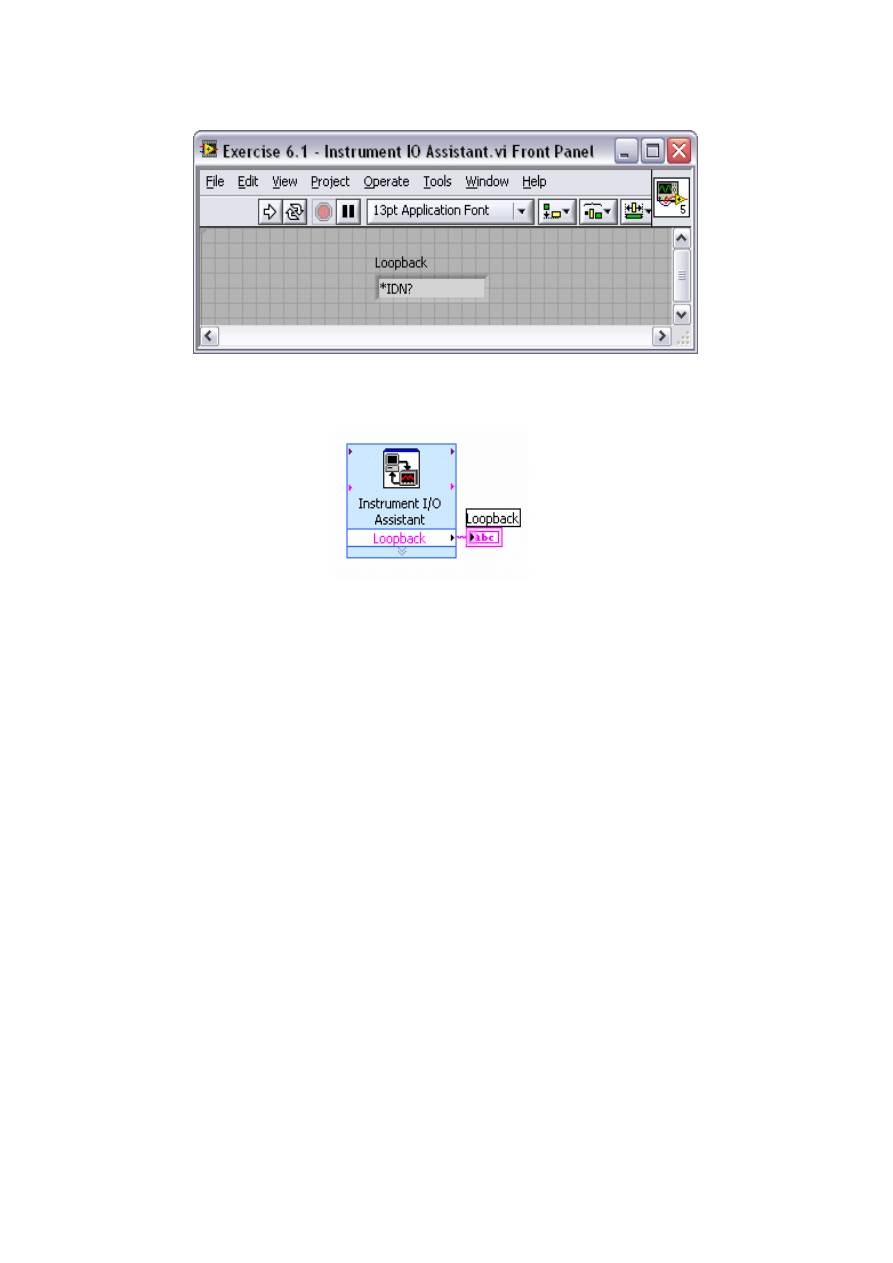
Exercise 6.1 – Loop back test with Instrument I/O Assistant
Note: This exercise uses the serial port and requires a serial cable and a wire. Most PCs
have a built in serial port available. The Instrument I/O Assistant can easily be used to
communicate with a GPIB device as well, but would require GPIB hardware instead of
the serial port.
Complete the following steps to configure the Instrument I/O Assistant to perform a
loopback test using the serial port.
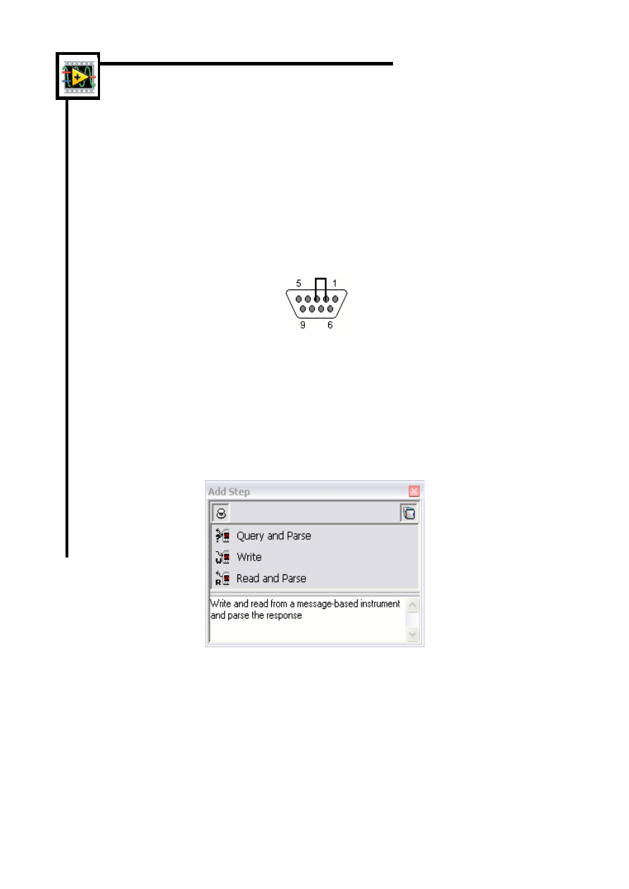
1. Connect the serial cable to the COM port of the computer.
2. Connect the transmission and receive lines of the serial cable by connecting pins 2 and
3, as shown below.
3. Open a blank VI from the Getting Started screen.
4. Place the Instrument I/O Assistant on the block diagram. Right-click to open the
functions palette and select Instrument I/O » Instrument I/O Assistant.
5. Open the Instrument I/O Assistant configuration dialog box by double-clicking on the
icon if it does not appear.
6. Select COM1 from the Select an Instrument drop-down box.
7. Click Add Step to create a new step and select Query and Parse.
8. Configure the Query and Parse Step:
a.
Type *IDN? in the Enter a Command field.
b. Name the output of the Instrument I/O Assistant by entering Loopback in the
Token name field.
c.
Click the “Run this Step” button to execute the loopback test.
d. Click the “Auto Parse” button to convert the raw data to ASCII.
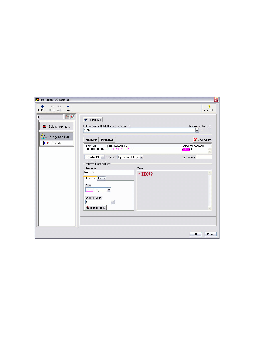
9. Click the OK button to exit the configuration window and generate the code.
10. Right-click the string output of the Instrument I/O Assistant and create an indicator.
11. Return to the front panel and run the VI. Observe the text in the indicator. Since we are
performing a loop back test the text of the indicator should match what command was entered
in the Instrument I/O Assistant. *IDN? is a standard command that returns device
information, but any text could have been used for a loop back test.
12. Save and close the VI.
(End of Exercise)
Solutions Section
Exercise 1.2:
Exercise 1.2 – Track C:
Exercise 1.2 – Track A and B:
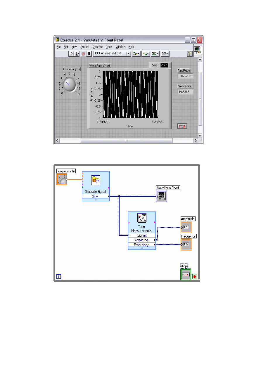
Exercise 2.1:
Exercise 2.1 – Track A, B, and C:
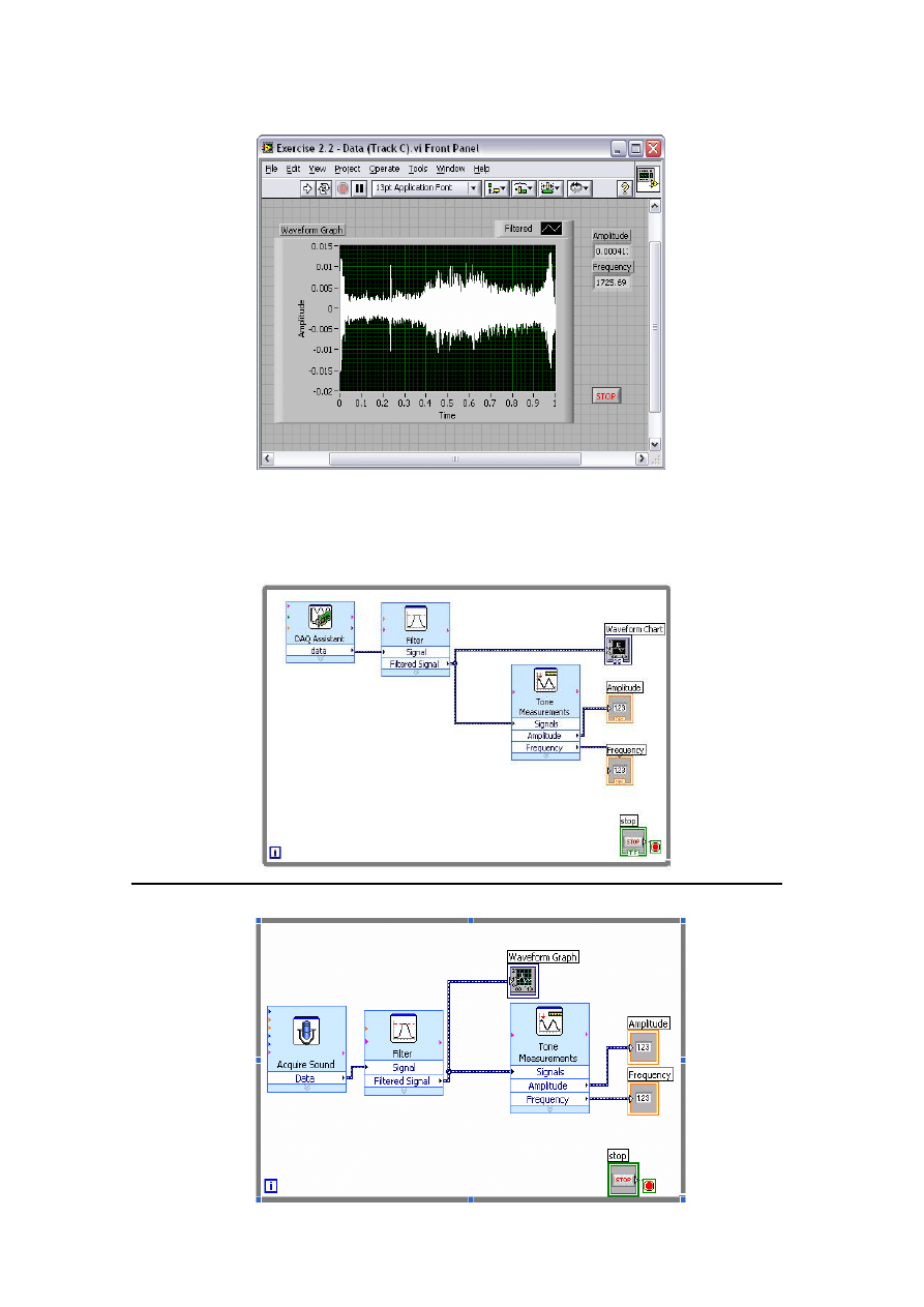
Exercise 2.2:
Exercise 2.2 – Track C:
Exercise 2.2 – Track A and B:
Note: Waveform Graphs and Charts have been
used interchangeably in Exercise 3.2 and 3.3.
Exercise 2.3:
Exercise 2.3 – Track C:
Exercise 2.3 – Track A and B:
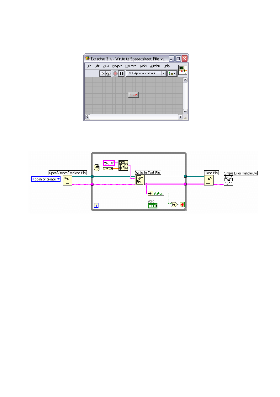
Exercise 2.4:
Exercise 2.4
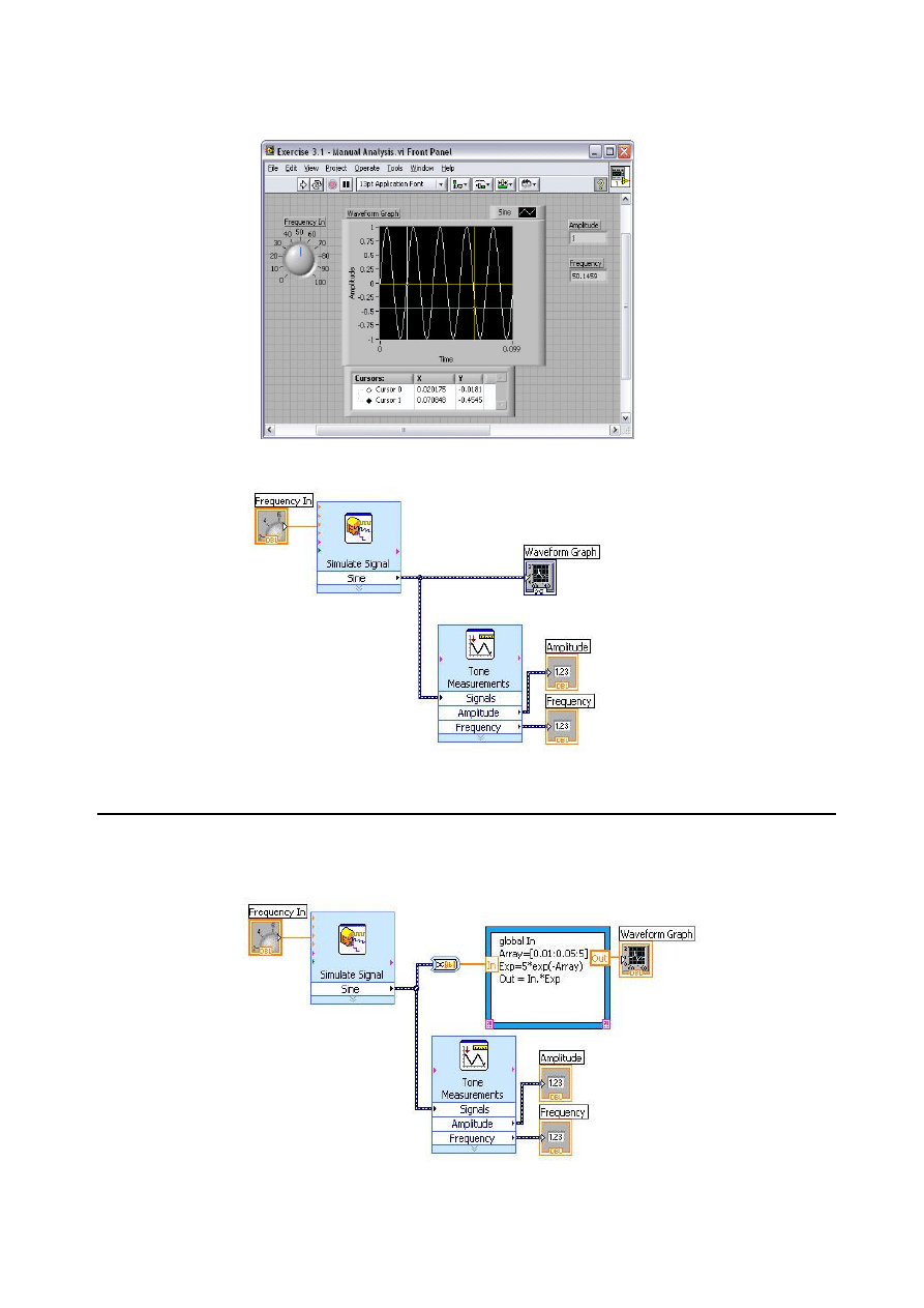
Exercise 3.1 and 3.2:
Exercise 3.2 – Track A, B, and C:
Exercise 3.1 – Track A, B, and C:
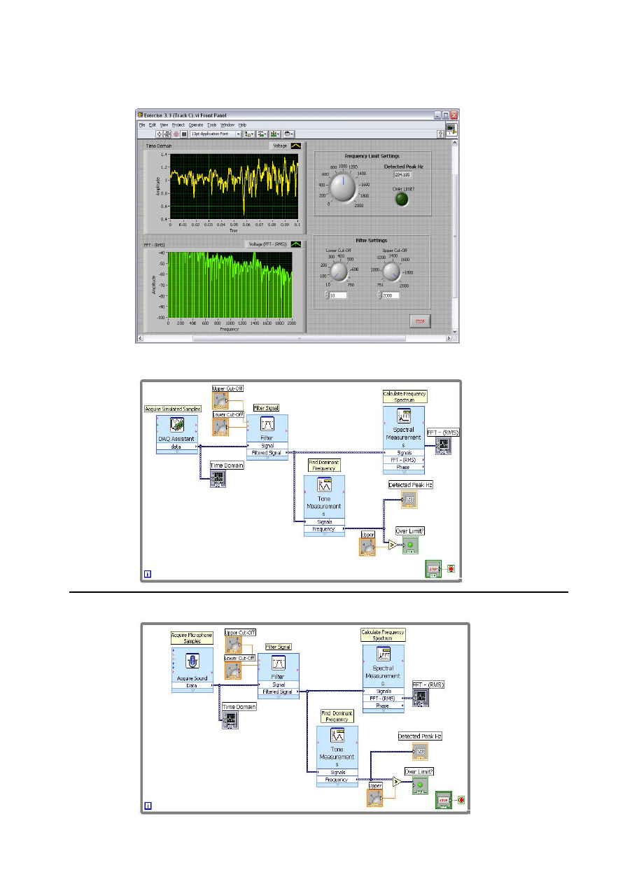
Exercise 3.3:
Exercise 3.3 – Track A and B:
Exercise 3.3 – Track C:
Exercise 4.1:
Exercise 4.1:
Exercise 4.2:
Exercise 4.2:
Exercise 5.1:
Exercise 5.1:
Exercise 6.1:
Exercise 6.1:
Wyszukiwarka
Podobne podstrony:
An Introduction To Olap In Sql Server 2005
Poisonous and Edible Mushrooms An Introduction to Mushrooms in Norway (2012)
Introduction to Literature in English Erasmus
Jay An Introduction to Categories in Computing [sharethefiles com]
Countdown to French Learn to Communicate in 24 Hours
Introduction to multivariate calibration in analytical chemistry
Network manipulation in a hex fashion An introduction to HexInject
Countdown to French Learn to Communicate in 24 Hours
ENGLISH TO PĀLI EXERCISES IN A K WARDER’S INTRODUCTION TO PALI
Introduction to VHDL
268257 Introduction to Computer Systems Worksheet 1 Answer sheet Unit 2
Introduction To Scholastic Ontology
Evans L C Introduction To Stochastic Differential Equations
Zizek, Slavoj Looking Awry An Introduction to Jacques Lacan through Popular Culture
Introduction to Lagrangian and Hamiltonian Mechanics BRIZARD, A J
Introduction to Lean for Poland
An Introduction to the Kabalah
Introduction to Apoptosis
więcej podobnych podstron