Characterization of Particle-Size Distribution in Soils with a Fragmentation Model

Marco Bittelli,* Gaylon S. Campbell and Markus Flury

ABSTRACT

to be best suited. The Shiozawa and Campbell model
divides the particle distribution into two parts domi-

Particle-size distributions (PSDs) of soils are often used to estimate

nated by primary (sand and silt) and secondary (clay)

other soil properties, such as soil moisture characteristics and hydraulic
conductivities. Prediction of hydraulic properties from soil texture

minerals, respectively. However, as pointed out by Bu-

requires an accurate characterization of PSDs. The objective of this

chan et al. (1993), the assumption of a lognormal distri-

study was to test the validity of a mass-based fragmentation model

bution in the clay fraction cannot be justified because

to describe PSDs in soils. Wet sieving, pipette, and light-diffraction

Shiozawa and Campbell (1991) had no data available

techniques were used to obtain PSDs of 19 soils in the range of 0.05

in that range.

to 2000

mm. Light diffraction allows determination of smaller particle

One of the latest developments in the study of PSDs

sizes than the classical sedimentation methods, and provides a high

in soils has focused on the use of fractal mathematics

resolution of the PSD. The measured data were analyzed with a mass-

to characterize particle sizes in soil (Turcotte, 1986;

based model originating from fragmentation processes, which yields

Tyler and Wheatcraft, 1992; Wu et al., 1993). However,

a power-law relation between mass and size of soil particles. It was

questions remain about the validity and applicability of

found that a single power-law exponent could not characterize the
PSD across the whole range of the measurements. Three main power-

fractal concepts to PSDs. There has been some discus-

law domains were identified. The boundaries between the three do-

sion about the proper use and definition of the term

mains were located at particle diameters of 0.51

6 0.15 and 85.3 6

“fractal” in the literature (Young et al., 1997; Pachepsky

25.3

mm. The exponent of the power law describing the domain be-

et al., 1997; Baveye and Boast, 1998). Different concepts

tween 0.51 and 85.3

mm was correlated with the clay and sand contents

of fractals are used, and these concepts lead to different

of the soil sample, indicating some relationship between power-law

interpretations of fractal dimensions obtained. There-

exponent and textural class. Two simple equations are derived to

fore it is essential to clearly specify the type of fractal

calculate the parameters of the fragmentation model of the domain

model used.

between 0.51 and 85.3

mm from mass fractions of clay and silt.

Particle- and aggregate-size distributions are often

rendered as cumulative functions, either as number of
particles larger than a certain diameter, or as mass

P

article-size distribution in soil is one of the more

smaller than a certain diameter. These cumulative distri-

fundamental soil physical properties. It is widely

bution functions have been analyzed with power-law

used for the estimation of soil hydraulic properties such

relations and the exponents interpreted as fractal di-

as the water-retention curve and saturated as well as

mensions. Tyler and Wheatcraft (1989, 1992) analyzed

unsaturated conductivities (Arya and Paris, 1981;

particle-size data ranging from 0.5- to 5000-

mm radii,

Campbell and Shiozawa, 1992). Generally, a conven-

and observed that the fractal power law was not valid

tional particle-size analysis involves the measurement

across the entire extent of particle sizes. It is expected

of the mass fractions of clay, silt, and sand. These frac-

that there are lower and upper limits to the validity

tions may be used to find the textural class using a

of fractal relations (Turcotte, 1986). Wu et al. (1993)

textural diagram, commonly in form of a textural trian-

measured PSDs down to 0.02-

mm radius by using light-

gle (e.g., Gee and Bauder, 1986). However, soil samples

scattering techniques, and found a power-law relation

that fall into a certain textural class may have consider-

between number of particles and particle radius valid

ably different PSDs. For example, the textural class of

across a range of particle radii with a lower cutoff be-

“clay” in the USDA classification scheme (Gee and

tween 0.05 and 0.1

mm and an upper cutoff between 10

Bauder, 1986) contains soil samples that vary in clay

and 5000

mm. Assuming that the exponent of a power-

content between 40 and 100%. The size definitions of

law relation is a fractal dimension, Wu et al. (1993)

the three main particle fractions of clay, silt, and sand,

found a dimension of D

5 2.8 6 0.1 for the four soils

used as diagnostic characteristics in most classification

studied and suggested that this might be a universal

schemes, are rather arbitrary, and they do not provide

value of an underlying structure. Kozak et al. (1996)

complete information on the soil PSD.

analyzed PSDs of 2600 soil samples and found that for

A more accurate description of texture is obtained

50% of the samples power-law scaling of particle num-

by defining a PSD function. Commonly, PSDs are re-

bers vs. size was not applicable across the whole range

ported as cumulative distributions, and different func-

of particle sizes between 2 and 1000

mm. The authors

tions have been proposed to fit experimental data. Bu-

indicate that power-law scaling might be applicable for

chan et al. (1993) fitted several of these models to

a narrower range of particle sizes, although this was not

experimental data and found the bimodal lognormal

analyzed in their study.

distribution proposed by Shiozawa and Campbell (1991)

Most applications of fractal concepts to particle- and

aggregate-size distributions are based on the fragmenta-

M. Bittelli, G.S. Campbell, and M. Flury, Department of Crop and

tion model of Matsushita (1985) and Turcotte (1986).

Soil Sciences, Washington State University, Pullman, WA 99164. Re-
ceived 26 Aug. 1998. *Corresponding author ([e-mail]).

Abbreviations: PSD, particle-size distribution; RMSE, root mean
square error.

Published in Soil Sci. Soc. Am. J. 63:782–788 (1999).

782

BITTELLI ET AL.: FRAGMENTATION MODEL TO CHARACTERIZE PARTICLE-SIZE DISTRIBUTION

783

Table 1. Soil classification, geological parent material, percentage of sand, silt and clay by weight, and organic C content for the 19 soils

used. Particle-size data were obtained by sieving and light-diffraction methods. Textural classes are according to the USDA classification.

Soils

Soil classification†

Geological parent material

Sand

Silt

Clay

OC§

%

Affoltern

Typic Hapludalf

moraine

47.4

48.5

4.1

2.2

Aeugst

Typic Hydraquent

fluvial deposits

38.7

55.6

5.7

1.9

Buelach

Typic Hapludalf

gravel deposits

57.2

40.4

2.4

2.2

Les Barges

Mollic/Aquic Udifluvent

fluvial deposits

74.2

25.5

0.3

1.0

Mettmenstetten

Lithic Ustorthent

moraine

55.6

40

4.4

0.4

Murimoos

Lithic Medihemist

fluvial deposits

69.9

29.6

0.5

1.0

Obermumpf

Lithic Rendoll

limestone

25.6

69.2

5.2

0.5

Obfelden

Typic Hydraquent

fluvial deposits

36.3

59.6

4.1

0.6

Palouse‡

Ultic Haploxeroll

loess

13.2

68.6

18.2

na¶

Reckenholz

Vertic/Typic Eutrochrept

moraine

23.8

70.7

5.5

1.3

Red Bluff‡

Ultic Palexeralfs

fluvial deposits

17.9

36.5

45.6

na

Rheinau

Arenic Eutrochrept

fluvial gravels

68.1

29.2

2.7

0.8

Royal‡

Ultic Haploxeroll

glaciofluvial sediments

30.7

63.1

6.2

na

Salkum‡

Xeric Palehumults

glacial drift

11.9

59.7

28.4

na

Walla Walla‡

Typic Haploxeroll

loess

8.3

78.4

13.3

na

Wetzikon 1

Lithic Ruptic-Alfic Eutrochrept

moraine

48.9

46.7

4.4

0.9

Wetzikon 2

Rendollic Eutrochrept

moraine

59.7

37.2

3.1

0.9

Wuelflingen

Vertic/Typic Eutrochrept

anthropogenic deposits

32.7

60.5

6.8

0.7

Zeiningen

Ultic Hapludalf

floess

40.5

55.4

4.1

0.4

† U.S. soil taxonomy.
‡ Soils from USA.
§ OC, organic C percentage by weight, determined with Walkley-Black method (Nelson and Sommers, 1982).
¶ na, not available.

dried at 105

8C, gently crushed, and passed through a 2-mm

In this model, the fragmentation of an initially intact

sieve. Each sample was tested for the presence of carbonates

particle into smaller particles leads to a power-law rela-

using cold 1 M HCl, and if carbonates were present, the sample

tion between (i) number or (ii) mass of particles as a

was treated with 0.5 M sodium acetate at 75

8C for at least 1 h.

function of particle size. These two types of fragmenta-

After acetate treatment, samples were washed with deionized

tion relations are known as number-based and mass-

water. The five soil samples from the USA were further pre-

based approaches (Turcotte, 1992). The power-law ex-

treated by destroying organic matter using H

2

O

2

(30%, w/w)

ponent of the number-based approach can be inter-

at 65

8C. The 14 Swiss soil samples were not pretreated for

preted as fractal dimension (Matsushita, 1985; Turcotte,

organic matter. The absence of pretreatment for organic mat-

1986). It is worth noting that the fragmentation model

ter could in some cases have affected the dispersion of particles
for the Swiss soils, leading to incomplete segregation, and

does not lead to a geometrical fractal with the fractal

therefore to an underestimation of small particle fractions.

dimensions confined between Euclidian dimensions.

Organic matter contents of the Swiss soils, determined with the

The sorting of particles by size in the fragmentation

Walkley-Black method (Nelson and Sommers, 1982), ranged

model results in fractal dimensions ranging theoretically

from 0.4 to 2.2% by weight (Table 1).

between the limits of 0 and 3 (Turcotte, 1986). Borkovec

After pretreatment, all samples were dried at 105

8C for 24

et al. (1993) experimentally determined fractal dimen-

h. Prior to particle-size analysis, all soil samples were dispersed

sions of fragmentation and surface areas of soil particles

in 1 g L

2

1

hexametaphosphate solution and shaken for 24 h

and found the two dimensions to be 2.8

6 0.1 and 2.4 6

to destroy aggregates. For the pipette analysis, samples were

0.1, respectively.

wet sieved with the hexametaphosphate solution at 1000-,

The objective of this study was to test the mass-based

500-, 250-, 125-, and 53-

mm mesh sizes. The material smaller

than 53

mm was then analyzed by the pipette method (Gee

fragmentation approach proposed by Turcotte (1986)

and Bauder, 1986). To obtain four size classes between 2 and

for characterizing PSDs, and to determine the range of

50

mm, sedimentation techniques based on Stoke’s law were

particle diameters where power-law scaling is applica-

used to obtain the following diameters:

,2, ,5, ,10, and ,20

ble. To test the general validity and the extent of power-

mm. For the light-scattering technique, the soil samples were

law scaling it is of fundamental importance to have

wet sieved down to a size of 250

mm for the Swiss soils and

data that span several orders of magnitude. Traditional

500

mm for the U.S. soils. The particles passing the smallest

sedimentation and hydrometer techniques for the mea-

sieve mesh were collected in a bucket, dried at 105

8C, and

surement of PSDs yield only limited data in the clay

subsequently analyzed by light diffraction. A 3-g aliquot of

fraction smaller than 2

mm. Light-scattering methods

the dried material was introduced into an ultrasonic bath unit

overcome this problem and provide data between 0.05

of a small-angle light-scattering apparatus (Malvern Master
Sizer MS20, Malvern, England) equipped with a low-power

to 1000

mm.

(2 mW) Helium-Neon laser with a wavelength of 633 nm as
the light source.

1

Suspension concentrations were adjusted to

MATERIALS AND METHODS

an obscuration of the primary beam of

≈

0.1 to 0.2%. The

Particle-Size Analysis

obscuration values were set to optimize between best signal/
noise ratio and negligible multiple scattering effects. If the

Nineteen soils were used in this study, five of them were

sample concentration is too low, the obscuration and the inten-

from the USA and 14 from Switzerland. The soils were chosen
such that they represent a wide variety of parent materials,
weathering conditions, and textures. Characteristic properties

1

Reference to company name does not reflect endorsement of

particular products by Washington State University.

of these soils are summarized in Table 1. All soil samples were

784

SOIL SCI. SOC. AM. J., VOL. 63, JULY–AUGUST 1999

sity of the scattered light are low, leading to noisy data. If the
sample concentration is too high, then the light scattered from
a particle may be scattered again by a second particle, causing
errors in the final particle-size analysis. Prior to measurement,
samples were dispersed by sonication in an ultrasonic bath
for 25 min. A focal length of 300 mm was used with an ordinary
Fourier Optics configuration, and a focal length of 45 mm was
used for the inverse Fourier Optics configuration. The inverse
configuration allows the accurate measurement of scattering
at high angles in order to correctly measure the very fine
particles (sizes down to 0.01

mm). Particle-size distribution

was obtained by fitting full Mie scattering functions for spheres
(Kerker, 1969).

Data Analysis

Soils are formed by weathering of geological parent mate-

rial. The weathering results in a fragmentation of the initial
solid rock or sediment. It has been recognized that the prod-

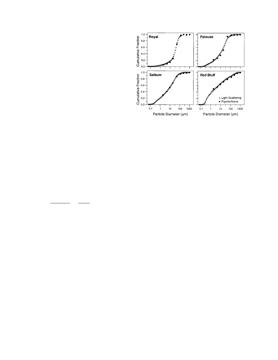
Fig. 1. Cumulative particle-size distributions for four soils obtained

ucts of fragmentation in nature can often be described with

by two different experimental methods.

fractal concepts. For different types of objects, a power-law
relation between the number and size of objects has been

shown below by our experimental data and discussed in the

proposed (Mandelbrot, 1982; Matsushita, 1985; Turcotte,

literature (Turcotte, 1992), the power-law relation given in

1986)

Eq. [2] has also a lower limit of validity. The radius R of

N(r

. R) 5 CR

2

D

[1]

particles satisfying Eq. [2] is confined between R

L,lower

,

R

, R

L,upper

.

where N(r

. R) is the number of objects per unit volume

The mass-based fragmentation approach was used to ana-

having a radius r larger than R, C is a constant of proportional-

lyze experimentally determined PSD data. The lower and up-

ity, and D is the fractal dimension. For soil particles, Turcotte

per limits R

L,lower

and R

L,upper

as well as the power-law exponent

(1986) and Tyler and Wheatcraft (1992) pointed out that it is

D

5 3 2 v were determined by the following procedure. A

generally more convenient to express the number-based power

linear regression was used to fit Eq. [2] on a log-log plot to

law (Eq. [1]) as a mass-based form. The mass-based approach

the experimental data. The entire range of experimental data

is compatible with data obtained from experimentation, where

was used first and the residuals were calculated. Subsequently,

usually mass fractions rather than number fractions are mea-

the upper- and lower-range data points were eliminated and

sured. The mass-based form of Eq. [1] is expressed as (Tur-

new residuals and root mean square errors (RMSE) were

cotte, 1986; Tyler and Wheatcraft, 1992)

calculated. In an iterative procedure, the RMSE error was
minimized by eliminating data points at the upper and

M(r

, R)

M

T

5

1

R

R

L,upper

2

v

[2]

lower boundaries.

where M(r

, R) is the mass of soil particles with a radius

RESULTS AND DISCUSSION

smaller than R, M

T

is the total mass of particles with radius

less than R

L,upper,

R

L,upper

is the upper size limit for fractal behav-

Comparison between Pipette and

ior, and v is a constant exponent. This power law can be

Light-Diffraction Methods

related to the fractal number relation by taking incremental
values as shown by Matsushita (1985) and Turcotte (1992).

Most of the textural data reported in the literature

Taking the derivatives of Eq. [1] and [2] with respect to the

have been measured by sedimentation techniques, such

radius R yields, respectively,

as hydrometer or pipette. It is therefore illustrative to
briefly compare experimental results obtained by pi-

dN

~ R

2

D

2

1

dR

[3]

pette and light-scattering methods. The results obtained

and

by the two techniques were in excellent agreement in
our study. Figure 1 shows a qualitative comparison be-

dM

~ R

v

2

1

dR

[4]

tween pipette and light-scattering methods for four soils.

Assuming a constant density of soil particles, the volume of

Experimental differences in the cumulative fraction at

a particle with radius r is proportional to its mass m, hence

a given particle size obtained by the two methods were

r

3

~ m; therefore, for incremental particle numbers and masses

in the order of 0.3 to 11.7%. Similar results were ob-

we have

tained by Wu et al. (1993), who found that sedimenta-

R

3

dN

~ dM

[5]

tion and light-scattering techniques were in good agree-

Substituting Eq. [3] and [4] into [5] gives (Turcotte, 1992)

ment for the majority of the soil samples used in their
experiment.

R

2

D

2

1

~ R

2

3

R

v

2

1

[6]

from which it follows that

Characterization of Particle-Size Distribution

D

5 3 2 v

[7]

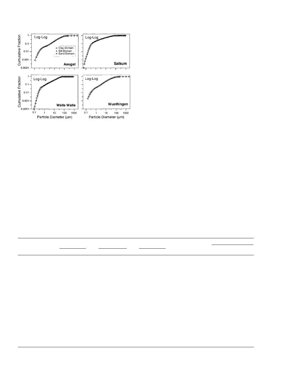
In Fig. 2, cumulative mass fractions are plotted as a

function of particle diameter on double logarithmic

Equation [7] relates the exponent v of the mass-based ap-
proach to the exponent D of the number-based approach. As

scale for four soils. The plots clearly show that a single

BITTELLI ET AL.: FRAGMENTATION MODEL TO CHARACTERIZE PARTICLE-SIZE DISTRIBUTION

785

ary was 0.51

mm and of the silt–sand domain boundary

was at 85.3

mm, with a coefficient of variation of 15 and

25%, respectively. The consistent occurrence of three
power-law domains in all 19 soils and the close agree-
ment of the domain scales indicate similarity between
the different soils, particularly when considering the
wide textural variability of the samples ranging from
0.3 to 46% clay. In a similar study on four soils, Wu et
al. (1993) also found three domains where a power law
was applicable, but the limits between the domains were
located at 0.05 to 0.1 and 10 to 5000

mm. The consistency

of the limits for the three domains needs therefore to
be investigated across a greater number of soils.

We denote the three fractal dimensions determined

in our study as D

clay

, D

silt

, and D

sand

. The fitted values of

the fractal dimensions obey in all cases the relation: D

clay

, D

silt

, D

sand

. In the clay domain, the fractal dimension

Fig. 2. Log-log plots of particle-size distributions for four soil samples.

ranged from 0.118 to 1.21, in the silt domain from 1.728

Symbols denote experimental data, solid lines denote model fits.

and 2.792, and in the sand domain from 2.839 to 2.998
(Table 2). These data are consistent with the limits of the

power law cannot describe the data across the entire

fragmentation approach given as 0

, D , 3 (Turcotte,

range of measured particle sizes. There is evidence that

1986). The generally high value of the coefficient of

different power laws apply for three domains in all of

determination R

2

shows that the fragmentation models

the 19 soils. The solid lines in Fig. 2 are the curves of

are good descriptions of the PSDs in the three domains.

Eq. [2] fitted to the different domains of particle sizes

Some soils showed poor power-law agreement in the

on the log-log plots.

sand domain (e.g., Obfelden and Reckenholz). Experi-

Optimized parameters of the fragmentation model

mental data in the sand as well as in the clay domain

together with the median particle diameter for all the

are limited by the experimental procedures, namely the

19 soils are shown in Table 2. The median diameter has

maximum particle size as allowed by the 2-mm sieve

been calculated from the measured PSDs by linearly

mesh and the minimum particle size determined by the

interpolating the 50% quantile (e.g., Sokal and Rohlfs,

light-scattering technique.

1995). The identified power-law domains separate the

The model used in the derivation of Eq. [2] is based

particle sizes in three classes, which we denote as clay,

on the fragmentation of an initially intact particle into

silt, and sand domains. The diameter boundaries be-

smaller particles (Matsushita, 1985; Turcotte, 1986). An

tween the clay and silt domains ranged from 0.33 to

intact cubical particle of size h is fragmented into eight

0.99

mm, and between silt and sand domains from 45.3

identical cubes of size h/2. Each of these smaller cubes
is further divided in cubes with size h/4, and so forth.

to 126.7

mm. The average of the clay–silt domain bound-

Table 2. Fragmentation fractal dimensions, median particle diameter, and cutoff boundaries, estimated from particle-size distribution

data obtained by the light-diffraction method for the 19 soils.

Clay domain

Silt domain

Sand domain

Silt domain

Median

Lower

Upper

Soils

D

clay

R

2

D

silt

R

2

D

sand

R

2

diameter d

50

boundary

boundary

mm

mm

mm

Affoltern

0.808

0.96

2.239

0.99

2.930

0.95

46.19

0.42

94.35

Aeugst

0.606

0.97

2.294

0.99

2.979

0.94

36.51

0.38

93.93

Buelach

0.596

0.96

2.122

0.99

2.898

0.96

60.01

0.99

98.41

Les Barges

0.808

0.99

1.768

0.99

2.839

0.98

74.96

0.53

124.58

Mettmenstetten

0.792

0.96

2.297

0.98

2.858

0.98

109.79

0.58

74.99

Murimoos

0.255

0.99

1.728

0.99

2.948

0.91

74.44

0.56

112.92

Obermumpf

0.701

0.96

1.801

0.99

2.974

0.98

30.96

0.40

56.93

Obfelden

1.210

0.97

2.152

0.98

2.969

0.85

24.86

0.40

69.98

Palouse

0.118

0.96

2.504

0.99

2.996

0.91

14.34

0.44

54.21

Reckenholz

0.789

0.96

2.238

0.99

2.998

0.81

29.22

0.40

71.58

Red Bluff

0.174

0.96

2.792

0.99

2.921

0.99

2.88

0.51

77.92

Rheinau

0.799

0.96

2.251

0.99

2.815

0.97

77.58

0.42

126.73

Royal

0.987

0.95

2.269

0.99

2.981

0.94

35.56

0.56

90.46

Salkum

0.214

0.97

2.618

0.98

2.953

0.99

8.18

0.63

45.31

Walla Walla

0.896

0.94

2.384

0.98

2.973

0.91

16.57

0.61

50.86

Wetzikon 1

0.796

0.99

2.249

0.99

2.931

0.98

50.04

0.38

98.57

Wetzikon 2

0.808

0.95

2.201

0.98

2.901

0.95

67.71

0.33

122.84

Wuelflingen

0.896

0.96

2.279

0.99

2.994

0.99

36.44

0.55

71.28

Zeiningen

0.795

0.96

2.182

0.99

2.991

0.96

30.85

0.34

101.71

Average

0.51

85.3

Standard deviation

0.15

25.3

Coefficient of variation, %

15

25

786

SOIL SCI. SOC. AM. J., VOL. 63, JULY–AUGUST 1999

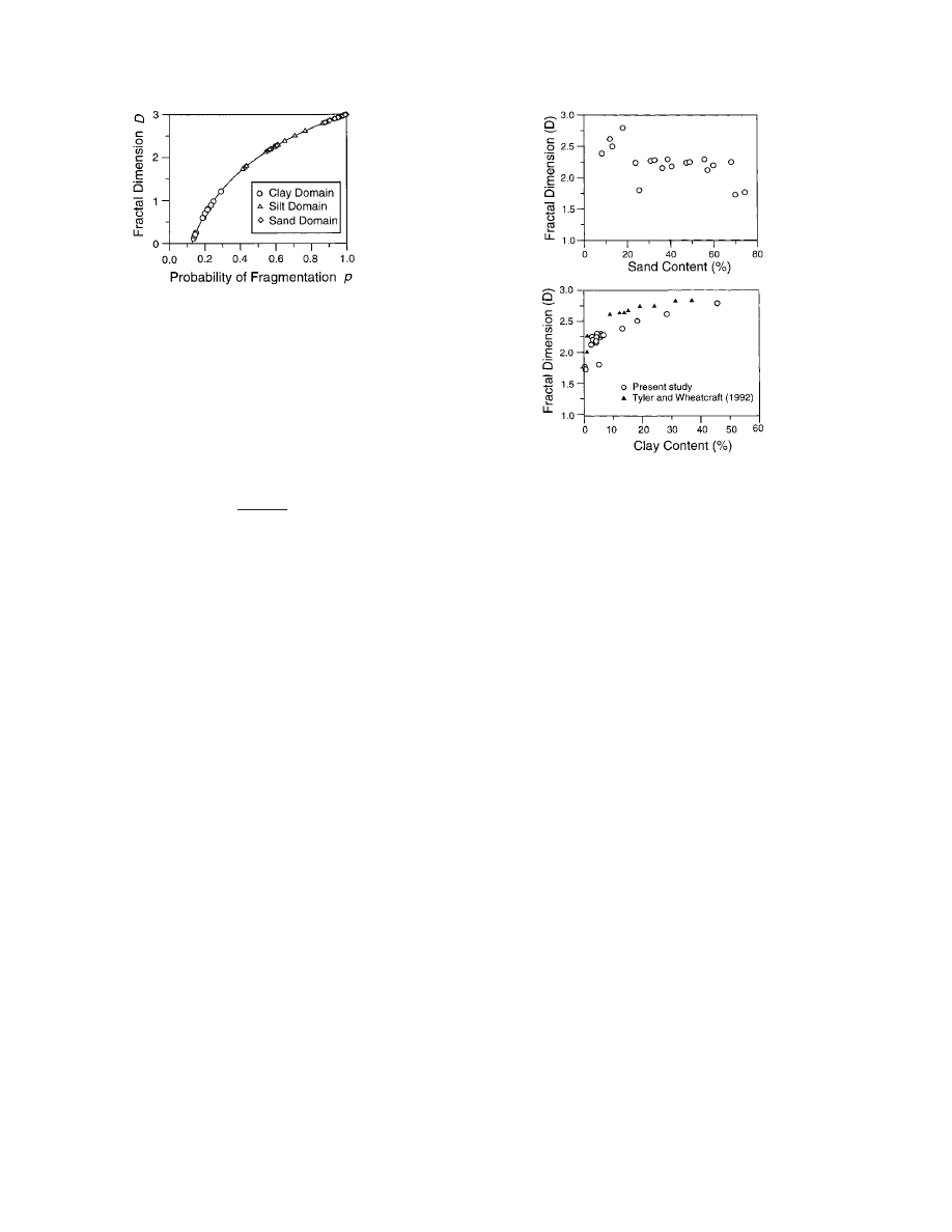
Fig. 3. Fragmentation fractal dimensions D and probabilities p of

fragmentation. The solid line represents Eq. [8], symbols are calcu-
lated with Eq. [8] from experimentally determined fractal di-
mensions.

The fragmentation of a cube has a certain probability
p, which is assumed to be constant for all orders of
fragmentation. A cube can maximally disintegrate into
eight smaller cubes (p

5 1) and minimally into one

smaller cube (p

5 1/8). As shown by Turcotte (1986),

the fragmentation probability p is related to the fractal

Fig. 4. Fragmentation fractal dimension of the silt domain D

silt

vs.

dimension D by

clay and sand percentage. Data from Tyler and Wheatcraft (1992)
were obtained from the entire range of the particle-size distribution
used in their study.

D

5

log(8p)

log 2

[8]

The fractal dimensions reported by Tyler and Wheatcraft

where the range of possible fractal dimensions is 0

,

(1992), plotted in this figure, were obtained by applying

D

, 3. Figure 3 shows a plot of Eq. [8] along with values

Eq. [2] to the entire range of the PSD data, which ranged

calculated from the analysis of our experimental data.

from 1 to 50

mm, 0.5 mm to 5 mm, and 16 mm to 1 mm

A scale-independent fragmentation process would have

for different data sets. Fractal dimensions given by Tyler

a constant fragmentation probability. Evidently, frag-

and Wheatcraft are therefore not directly comparable

mentation probabilities varied across almost the entire

with our D

silt

, but nevertheless, Fig. 4 shows a trend

range of 1/8

, p , 1. It is interesting that the fractal

between the D value and the clay and sand contents.

dimensions for the three domains are typically D

clay

,

The fractal dimension increases with clay content, and

D

silt

, D

sand

. It appears that for the 19 soils studied, the

decreases with sand content. These results suggest that

probability of fragmentation is scale dependent, and

the power-law relation of Eq. [2] can be used to charac-

in particular it decreases with decreasing size of the

terize PSD in soils, and may be an alternative to the

particles. There is experimental evidence that fragmen-

conventionally used approaches, such as the lognor-

tation of soil and sediment aggregates is scale dependent

mal distribution.

(Perfect et al., 1993; Rasiah et al., 1993). Larger aggre-
gates tend to fracture more easily than smaller aggre-

Calculation of Parameters of the Fragmentation

gates (Perfect, 1997). Considering soil particles as prod-

Model from Mass Fractions of Clay and Silt

ucts of a fragmentation process, our results are in
qualitative agreement with observations from aggregate

It is evident that no single power law can characterize

the PSD of a soil across the entire scale usually measured

failure studies.

Particle-size distribution measurements are strongly

in a particle-size analysis. For the majority of the sam-
ples, 46 to 86% (with an average of 71%) of the total

influenced by the experimental methods of dispersion
of the soil particles. The dispersion itself can be regarded

mass is carried by particles with diameters between 0.51
and 85.3

mm, the silt domain of the distribution. On a

as a fragmentation process. Organic matter increases
aggregate stability and hence leads to less fragmentation

log-log scale, the PSD of the silt domain is a straight
line and is therefore characterized by two parameters,

(Rasiah et al., 1993). Therefore the omission of organic
matter removal in the Swiss soils probably leads to less

the intercept and the slope of the power-law distribu-
tion. If we know any two points on this line, we can

dispersion of smaller particles. This explains the smaller
clay fractions determined in the Swiss soils compared

calculate the model parameters of the silt domain. As
Table 2 shows, the USDA boundaries between clay and

with the U.S. soils (Table 1). Based on the fragmentation
model, we would also expect smaller fractal dimensions

silt (2

mm), and between silt and sand (50 mm) are within

the silt domains for all 19 soils. Therefore we can use

for the clay fraction of the Swiss soils compared with
the U.S. soils; however, there is no evidence that this

these standard particle-class fractions to calculate the
two parameters of a power-law particle-size distribution

is the case (Table 2).

Following Tyler and Wheatcraft (1992), D

silt

vs. clay

in the silt domain. As the second parameter besides
the fractal dimension D we choose the median particle

and sand fraction was plotted in Fig. 4 to demonstrate
the relation between fractal dimension and soil texture.

diameter d

50

of the PSD. The median particle diameter

BITTELLI ET AL.: FRAGMENTATION MODEL TO CHARACTERIZE PARTICLE-SIZE DISTRIBUTION

787

CONCLUSIONS

There is evidence that cumulative PSDs in soils follow

a power-law distribution, consistent with a fractal frag-
mentation model. The mass-based approach suggested
by Matsushita (1985) and Turcotte (1986) showed good
agreement between the fractal model and our experi-
mental data. Three main domains—a clay, silt, and sand
domain—were identified where power-law scaling was
applicable. The limits between the domains were rela-
tively constant for different soil types, but do not coin-
cide with the traditional boundaries between clay, silt,
and sand. Fragmentation fractal dimensions of the three
domains increased in the order: clay

, silt , sand do-

main. A method is imposed to estimate the parameters
of the fragmentation model of the PSD in the silt domain
from standard textural data of clay, silt, and sand
fractions.

ACKNOWLEDGMENTS

We thank Alan Busacca and Sandra Lilligren for assistance

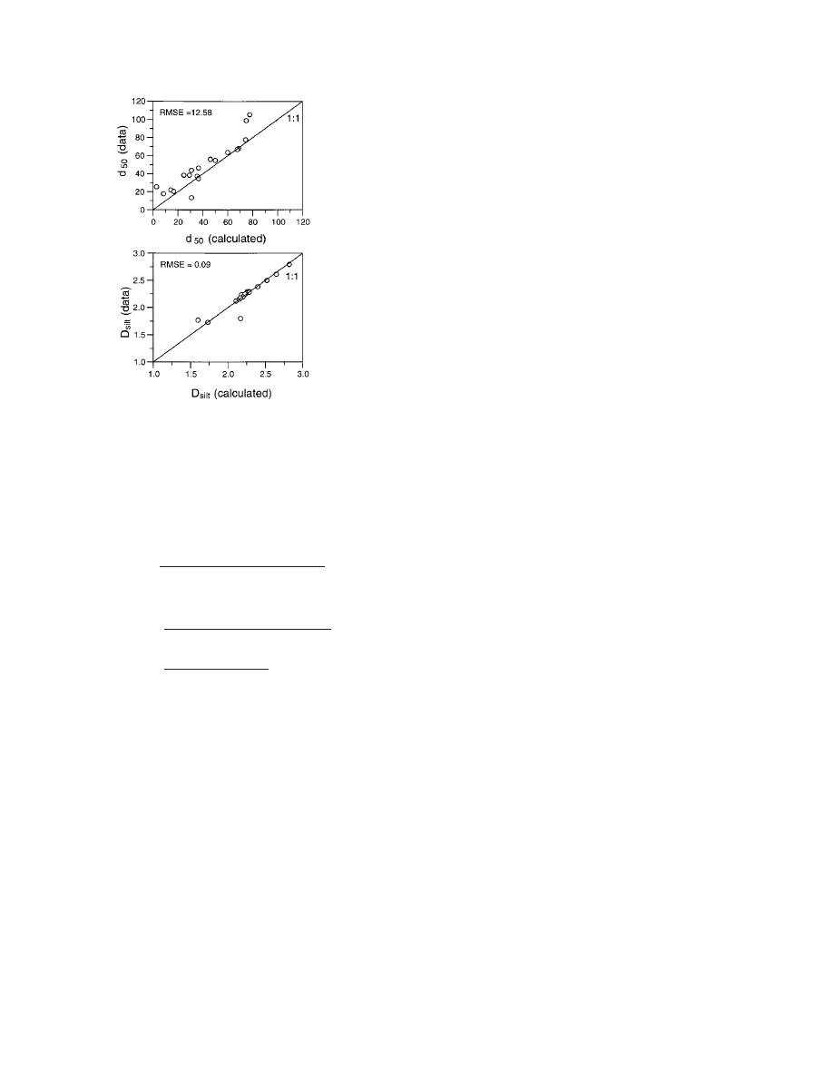
Fig. 5. Experimental and calculated values of median diameter d

50

during the laboratory analyses. The manuscript benefitted

and of fragmentation fractal dimension of the silt domain D

silt

for

from fruitful discussions with Claudio O. Stockle, Sally D.

all 19 soils used in this study. Calculated values are from Eq. [9]

Logsdon, and Philippe Baveye.

and [10]. RMSE is the root mean square error.

REFERENCES

is chosen because it is often used in empirical relations

Arya, L.M., and J.F. Paris. 1981. A physico-empirical model to predict

to predict other soil properties, and as such is a useful

the soil moisture characteristic curve from particle-size distribution

parameter to know. The median particle diameter d

50

and bulk density data. Soil Sci. Soc. Am. J. 45:1023–1030.

and the fractal dimension of the silt domain D

silt

can be

Baveye, P., and C.W. Boast. 1998. Concepts of “fractals” in soil sci-

ence: Demixing apples and oranges. Soil Sci. Soc. Am. J. 62:

calculated from standard textural data as follows

1469–1470.

Borkovec, M., Q. Wu, G. Degovics, P. Laggner, and H. Sticher. 1993.

d

50

5 exp

1

(2

2 D

silt

) log 2

2 log(m

clay

)

3

2 D

silt

2

[9]

Surface area and size distributions of soil particles. Colloids Surf.
Physicochem. Eng. Aspects 73:65–76.

Buchan, G.D., K.S. Grewal, and A.B. Robson. 1993. Improved models

and

of particle-size distribution: An illustration of model comparison
techniques. Soil Sci. Soc. Am. J. 57:901–908.

D

silt

5 3 2

log(m

silt

1 m

clay

)

2 log(m

clay

)

log 50

2 log 2

Campbell, G.S., and S. Shiozawa. 1992. Prediction of hydraulic proper-

ties of soils using particle-size distribution and bulk density data.
p. 317–328. In M.Th. van Genuchten, F.J. Leij, and L.J. Lund.

5 3 2

log(1

1 m

silt

/m

clay

)

log 25

[10]

(ed.) Indirect methods for estimating the hydraulic properties of
unsaturated soils. Univ. of California, Riverside.

Gee, G.W., and J.W. Bauder. 1986. Particle-size analysis. p. 383–411.

where m

clay

and m

silt

are the mass fractions of clay and silt,

In A. Klute (ed.) Methods of soil analysis. Part 1. 2nd ed. Agron.

log is the natural logarithm, and the median diameter d

50

Manag. 9. ASA and SSSA, Madison, WI.

Kerker, M. 1969. The scattering of light and other electromagnetic

is given in micrometers. Note that the median d

50

in Eq.

radiation. Academic Press, New York.

[9] is a non-log-transformed parameter. Mass fractions

Kozak, E., Y.A. Pachepsky, S. Sokolowski, Z. Sokolowska, and W.

of clay, silt, and sand are readily available for many

Stepniewski. 1996. A modified number-based method for estimat-

soils, and from these data the median diameter and

ing fragmentation fractal dimensions of soils. Soil Sci. Soc. Am.

the fractal dimension of the silt domain can then be

J. 60:1291–1297.

Mandelbrot, B.B. 1982. The fractal geometry of nature. Freeman and

computed with Eq. [9] and [10]. Note that in the deriva-

Co., San Francisco.

tion of Eq. [9] and [10] we assumed the USDA textural

Matsushita, M. 1985. Fractal viewpoint of fracture and accretion. J.

definition; for other classification schemes, the equa-

Phys. Soc. Jpn. 54:857–860.

tions have to be adapted accordingly.

Nelson, D.W., and L.E. Sommers. 1982. Total carbon, organic carbon,

and organic matter. p. 539–579. In A.L. Page (ed.) Methods of

We tested the validity of the two equations with our

soil analysis. Part 2. 2nd ed. Agron. Monogr. 9. ASA and SSSA,

19-soil data set. In Fig. 5, experimental d

50

and D

silt

values

Madison, WI.

(Table 2) are plotted vs. values calculated based on

Pachepsky, Y.A., D. Gime´nez, S. Logsdon, R.R. Allmaras, and E.

standard particle-size fractions using Eq. [9] and [10].

Kozak. 1997. On interpretation and misinterpretation of fractal

There is a good agreement between experimental and

models: A reply to “Comment on number-size distributions, soil
structure, and fractals”. Soil Sci. Soc. Am. J. 61:1800–1801.

calculated values, particularly for D

silt

. The RMSE in

Perfect, E. 1997. Fractal models for the fragmentation of rocks and

Fig. 5 shows that the d

50

is not estimated as well as the

soils: A review. Eng. Geology 48:185–198.

D

silt

, and generally the model tends to underestimate

Perfect, E., B.D. Kay, and V. Rasiah. 1993. Multifractal model for

the experimental value. The estimation of the fractal

soil aggregate fragmentation. Soil Sci. Soc. Am. J. 57:896–900.

Rasiah, V., B.D. Kay, and E. Perfect. 1993. New mass-based model

dimension is well performed by Eq. [10].

788

SOIL SCI. SOC. AM. J., VOL. 63, JULY–AUGUST 1999

for estimating fractal dimensions of soil aggregates. Soil Sci. Soc.

Tyler, S.W., and S.W. Wheatcraft. 1989. Application of fractal mathe-

matics to soil water retention estimation. Soil Sci. Soc. Am. J.

Am. J. 57:891–895.

Shiozawa, S., and G.S. Campbell. 1991. On the calculation of mean

53:987–996.

Tyler, S.W., and S.W. Wheatcraft. 1992. Fractal scaling of soil particle

particle diameter and standard deviation from sand, silt, and clay
fractions. Soil Sci. 152:427–431.

size distributions: analysis and limitations. Soil Sci. Soc. Am. J.
56:362–369.

Sokal, R.R., and F.J. Rohlfs. 1995. Biometry, 3rd ed. Freeman and

Co., New York.

Wu, Q., M. Borkovec, and H. Sticher. 1993. On particle-size distribu-

tions in soils. Soil Sci. Soc. Am. J. 57:883–890.

Turcotte, D.L. 1986. Fractals and fragmentation. J. Geophys. Res.

91:1921–1926.

Young, I.M., J.W. Crawford, A. Anderson, and A. McBratney. 1997.

Comment on number-size distributions, soil structure, and fractals.

Turcotte, D.L. 1992. Fractals and chaos in geology and geophysics.

Cambridge Univ. Press, Cambridge, UK.

Soil Sci. Soc. Am. J. 61:1799–1800.

Measuring Saturated Hydraulic Conductivity using a Generalized Solution

for Single-Ring Infiltrometers

L. Wu,* L. Pan, J. Mitchell, and B. Sanden

ABSTRACT

meter is a combination of both vertical and horizontal
flow (Tricker, 1978). A method to calculate the K

s

from

Saturated hydraulic conductivity is a measure of the ability of a

data obtained from a pressure or ring infiltrometer for

soil to transmit water and is one of the most important soil parameters.
New single-ring infiltrometer methods that use a generalized solution

both early-time and steady-state infiltration was devel-

to measure the field saturated hydraulic conductivity (K

s

) were devel-

oped by Reynolds and Elrick (1990), Elrick and Rey-

oped and tested in this study. The K

s

values can be calculated either

nolds (1992), and Elrick et al. (1995). Their steady-

from the whole cumulative infiltration curve (Method 1) or from

state method uses a shape factor that was numerically

the steady-state part of the cumulative infiltration curve by using a

calculated based on Gardner’s (1958) relationship be-

correction factor (Method 2). Numerical evaluation showed that the

tween hydraulic conductivity and matric pressure head.

K

s

values calculated from the simulated infiltration curves of represen-

Groenevelt et al. (1996) further extended this concept

tative soil textural types were in the range of 87 to 130% of the real

by developing a method to define the critical time that

K

s

values. Field infiltration tests were conducted on an Arlington fine

separates early-time and steady-state infiltration.

sandy loam (coarse-loamy, mixed, thermic, Haplic Durixeralfs). The

By applying scaling theory, Wu and Pan (1997) devel-

geometric means of the K

s

values calculated from the field-measured

infiltration curves by Method 1 and Method 2 were not significantly

oped a generalized solution for single-ring infiltromet-

different. The geometric mean of the K

s

calculated from the detached

ers. Wu et al. (1997) showed further that the infiltration

core samples, however, was about twice that of the K

s

calculated from

rate of a single-ring infiltrometer was approximately f

the infiltration curves, which was consistent with earlier findings.

times greater than the one-dimensional (1-D) infiltra-

Unlike the earlier approaches, Method 1 calculates K

s

values from

tion rate for the same soil, where f is a correction factor

the whole infiltration curve without assuming a fixed relationship

that depends on soil initial and boundary conditions and

(

a 5 K

s

/

f

m

) between saturated hydraulic conductivity and matric

ring geometry. For a relatively small ponded head, the

flux potential

f

m

.

1-D final infiltration rate of a field soil is approximately
equal to the field saturated hydraulic conductivity (K

s

),

which is valuable information for computer modeling,

S

aturated hydraulic conductivity is an important

as well as for irrigation management. The objectives of

soil parameter that measures the ability of a soil to

this research were (i) to develop alternative methods

transmit water. Measurement of field saturated hydrau-

to calculate K

s

by best fit of a generalized solution to

lic conductivity (K

s

) is often done by borehole permea-

the infiltration curves that are measured by single-ring

meters (Amoozegar and Warrick, 1986; Elrick and

infiltrometers, and (ii) to compare and evaluate K

s

val-

Reynolds, 1992). In many cases, however, measurement

ues calculated from infiltration curves of single-ring in-

of the soil surface K

s

is essential, especially in infiltra-

filtrometers with those measured by the single head

tion-related applications, such as irrigation manage-

(SH) method (Elrick and Reynolds, 1992) and detached

ment.

soil core samples (Klute and Dirksen, 1986).

Ring infiltrometers are often used for measuring the

water intake rate at the soil surface. Water flow from

THEORY

a single-ring infiltrometer into soil is a three-dimen-

A generalized infiltration equation developed by Wu and

sional (3-D) problem (Reynolds and Elrick, 1990). The

Pan (1997) has essentially the same form as the truncated

total flow rate into the soil from a single-ring infiltro-

Philip (1957) model of vertical infiltration. We propose here
to measure infiltration curves in the field and then utilize the
generalized equation to fit to the data in order to obtain

L. Wu, Dep. of Environmental Sciences, Univ. of California, River-
side, CA 92521; L. Pan, Earth Sci. Div., Lawrence Berkeley National

the relevant parameters for estimating K

s

. The generalized

Lab., Univ. of California, Berkeley, CA 95720; J. Mitchell, Kearney

equation (Wu and Pan, 1997) is

Agri. Center, Univ. of California, Parlier, CA 93648; and B. Sanden,

i/i

c

5 a 1 b(t/T

c

)

2

0.5

[1]

Univ. of California Coop. Ext., Kern County, Bakersfield, CA 93307.
Received 8 June 1998. *Corresponding author ([e-mail]).

Abbreviations: SH, single head.

Published in Soil Sci. Soc. Am. J. 63:788–792 (1999).